FLAMINGO: Fast Low-rAnk Matrix completion algorithm for reconstructINg high-resolution 3D Genome Organizations

!UPDATE (04/22/2024): FLAMINGOrLite

Lite version of FLAMINGO, high-resolution 3D chromosome structures reconstruction based on Hi-C.

https://github.com/JiaxinYangJX/FLAMINGOrLite/

Differences between FLAMINGOrLite and FLAMINGOr

1. FLAMINGOrLite doesn't support iFLAMINGO
2. FLAMINGOrLite is faster and more memory-efficient
3. FLAMINGOrLite is more user-friendly and fixed bugs in FLAMINGOr

Gallery

The 3D structures for chromosome 1-4 in 5-kb resolution in GM12878. The 3D structures for all 23 chromosomes could be found here.

An orbiting chromosome 1 on Youtube

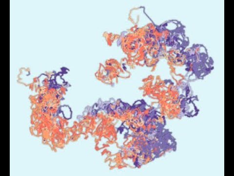
The 3D genome structure for chromosomes 1-4 in 1-kb resolution. The 3D structures for all 23 chromosomes could be found here.

Summary

We developed FLAMINGO to reconstruct the high-resolution 3D genome structures based on the chromatin contact maps with high scalability. By integrating the 1D epigenomics dataset, the integrative version of FLAMINGO (iFLAMINGO) is able to make cross-cell-type predictions and reconstruct high-resolution 3D structures from low-resolution contact maps.

Introduction

FLAMINGO takes cell-type specific distance matrices generated by Hi-C as inputs. By applying the low-rank matrix completion method on the observed distance matrices, an accurate prediction of 3D coordinates of DNA fragments is made. By further integrating the 1D epigenomics dataset in the target cell-type and the Hi-C data in the source cell-type, the integrative version of FLAMINGO,iFLAMINGO, is able to make cross cell-type predictions in the target cell-type. iFLAMINGO is also able to reconstruct high-resolution 3D structures from low-resolution contact maps by integrating the high-resolution 1D epigenomics dataset and low-resolution Hi-C data.

Dependencies

The implementation of the algorithm is based on bedtools and R 3.5.1. It depends on five R packages: strawr(0.0.9), parallel, mgcv(1.8-24), data.table (1.14.2) and Matrix(1.2-14).

Installation of the FLAMINGOr package

The R package for FLAMINGO (FLAMINGOr) can be installed through Github using devtools:

install.packages("devtools")
library(devtools)
install_github('wangjr03/FLAMINGO/FLAMINGOr',ref='HEAD')

Input data

Three standard formats of chromatin interaction data are supported: .hic, .mcool and the sparse matrix format.

Reconstruct the 3D genome structure with FLAMINGOr

The main function of FLAMINGO can be utilized as follow:

library(Matrix)
flamingo.main_func_large(
       hic_data_low,
       file_format,
       domain_res,
       frag_res,
       chr_size,
       chr_name,
       normalization,
       downsampling_rates,
       lambda,
       max_dist,
       nThread,
       alpha = -0.25,
       max_iter = 500,
       hic_data_high = NULL,
       norm_low = NULL,
       norm_high = NULL,
       n_row = 45000
     )

Arguments:

hic_data_low: The input chromatin interaction data in .hic format, .mcool format or sparse matrix format.

file_format: Foramt of the input chromatin interaction data. Could be .hic, .mcool or sparse matrix format.

domain_res: Size of the domains in bps, e.g. 1e6.

frag_res: Size of the fragment in bps, e.g. 5e3.

chr_size: Size of the chromosome in bps.

chr_name: Name of the chromosome, e.g. chr1.

normalization: Normalization method.

downsampling_rates: Fraction of contacts to be used for the reconstruction.

lambda: Lagrangian coefficient.

max_dist: The maximum allowed distance between two consecutive points.

nThread: Number of threads available for the reconstruction.

alpha: Conversion factor between the interaction frequency and the pairwise distance. default -0.25.

max_iter: The maximum number of iterations for the assembling algorithm. default 500.

hic_data_high: Optional. The high-resolution HiC data in sparse matrix format. Only required if the file_format is 'sparse matrix'.

norm_low: Optional. The normalization vector for the low-resolution Hi-C data. Only required if the file_format is 'sparse matrix'.

norm_high: Optional. The normalization vector for the high-resolution Hi-C data. Only required if the file_format is 'sparse matrix'.

n_row: Optional. The number of rows to use the large matrix format. Reduce the number if the memory is limited. default to 45000 rows.

Example code:
Taking Hi-C data in GM12878 '4DNFI1UEG1HD.hic' as an example (can be downloaded here), the following commands reconstruct the 3D genome structure of chromosome 1 in 5kb resolution. The whole process should take less than 30 minutes.

library(FLAMINGOr)
library(GenomicFeatures)
library(Matrix)
all_size <- getChromInfoFromUCSC("hg38")
chr_name ='chr1'
chr_size = all_size[all_size$chrom==chr_name,2]
res = flamingo.main_func_large(hic_data_low='../4DNFI1UEG1HD.hic',
                       file_format='hic',
                         domain_res=1e6,frag_res=5e3,
                         chr_size=chr_size,
                         chr_name=chr_name,
                         normalization='KR',
                         downsampling_rates=0.75,
                         lambda=10,max_dist=0.01,nThread=30,n_row=30000)

output data format

A data frame with four columns containing the fragment id (the first column) and the 3D coordinates (the other three columns) will be returned.

visualize the 3D genome structure using ParaView

ParaView is an open-source, multi-platform data analysis and visualization application. To visualize the 3D genome structure using FLAMINGO, the user need to convert the 3D coordinates into a .vtk file and use the ParaView software to visualize the structure. In the FLAMINGOr package, a write.vtk function is provided for such conversion using the command below:

write.vtk(points=res[,-1],lookup_table=rep(1,dim(res)[1]),name='chr1 5kb 3D structure',opt_path='./chr1_5kb.vtk')

Arguments:

points: 3D coordinates predicted by FLAMINGO in the x,y,z format.

lookup_table: The annotation of each point, could be labels or scores, i.e. the compartment PC scores.

name: output file name annotated within the file.

opt_path: output file path including the file name.

Stand-alone Scripts of FLAMINGO

The stand-alone scripts for all steps of FLAMINGO are provided below. The stand-alone version is especially useful when users have access to HPC, which can run hundreds of small jobs in parallel.

Input data

The algorithm takes two kinds of datasets as inputs: (1) If the user simply wants to reconstruct the 3D genome structure from the observed Hi-C contact maps from experiments, only the pairwise interaction frequency matrices are required. (2) If the user wants to make cross cell-type predictions or predict high-resolution structures from the low-resolution contact maps (i.e. iFLAMINGO), the cell-type specific epigenomics data, e.g. DNase-seq data, are required. The pairwise interaction frequency matrices generated by Hi-C can be downloaded from GEO (GSE63525) and the cell-type specific DNase-seq data can be downloaded from the Roadmap epigenomic consortium. Descriptions of the data are listed below:

1. The interaction frequency matrix: The interaction frequency matrix under a given resolution is summarized in the sparse matrix format. The associated KR normalization factors should also be included in the same directory. Taking Hi-C for example, the interaction frequency data should have three columns:

col	abbrev	type	description
1	Frag.id.1	integer	Index of the first DNA anchor
2	Frag.id.2	integer	Index of the second DNA anchor
3	IF	float	Hi-C interaction frequency

2. The cell-type specific DNase-seq data: The cell-type specific DNase-seq data should be stored in the bedGraph format with at least four columns. This input is only required by iFLAMINGO and could be ignored for FLAMINGO.

col	abbrev	type	description
1	chr	char	Name of the chromosome
2	start	integer	Start of the DNA fragment
3	end	integer	End of the DNA fragment
4	signal	float	DNase-seq signal strength

Description of scripts

The pipeline of the algorithm consists of eight pieces, including data preprocessing and modeling. A wrapper is provided to run the whole pipeline for each task and the user only needs to provide the path to the data. A detailed description of each piece is provided.

Wrapper and sample scripts for large scale applications
process_data_wrapper.sh : preprocess data, including step 1-6 introduced below. process_data_wrapper.sh: <path to 5kb-resolution Hi-C directory> <path to 1mb-resolution Hi-C directory> .
A sample * .sbatch * file to run the model on slurm-based HPC using job array is provided (* 7_resoncstruct_model_*_.sb *).

Scripts

1. 1_preprocess_HiC.R: This script normalizes Hi-C interaction frequencies and converts them to pairwise distances. The normalization is based on the KR normalization provided by Rao et al (2014). The normalized interaction frequencies are then transformed to the pairwise distances using the exponential transformation with \alpha =-0.25. The normalized interaction frequency matrix and distance matrix are stored as .Rdata files for later use.
   Command line usage: Rscript 1_preprocess_HiC.R <path to the folder containing the Hi-C data> <output path (define the working directory)>
   Notes: The parameter path to the folder containing the Hi-C data’ refers to the directory containing raw interaction frequency results AND KR normalization parameter files.
   

2. 2_generate_fragment_data.R: This script divides the entire chromosome into large DNA domains,e.g. 1 mb. The interaction frequency matrices and distance matrices are generated for each domain by further dividing domains into small DNA fragments, i.e. 5kb. The intra-domain interaction frequency matrices and distance matrices are used for the reconstruction of intra-domain structures.
   Command line usage: Rscript 2_generate_fragment_data.R <path to the working directory> <chromosome name, i.e. chr1>

3. 3_generate_fragment_DNase.R: This script generates the genomic location for all 5kb DNA fragments, which will be used for DNase integration and the downstream biological analysis. This part is only used by iFLAMINGO and could be skipped if no epigenomics data is required.
   Command line usage: Rscript 3_generate_fragment_DNase.R <path to the working directory> <chromosome name, i.e. chr1>

4. 4_generate_DNase_profile.R: This script generates the averaged DNase signal for each DNA fragment. This part is only used by iFLAMINGO and could be skipped if no epigenomics data is required.
   Command line usage: Rscript 4_generate_DNase_profile.R <path to the working directory> <path to the DNase bedgraph file>

5. 5_impute_DNase_dist.R: This script predicts the pairwise distance using the DNase signals of two DNA fragments and the 1D genomic distances based on a pre-trained regression model. This part is only used by iFLAMINGO and could be skipped if no epigenomics data is required.
   Command line usage: Rscript 5_impute_DNase_dist.R <path to the working directory>

6. 6_genereate_backbone_data.R: This script processes low-resolution Hi-C data, i.e. 1 mb-resolution, for the reconstruction of the domain-level structures. The method of normalization is the same as step 1.
   Command line usage: Rscript 6_genereate_backbone_data.R <path to the 5kb-resultion Hi-C data> <the working directory> <chromosome index>

7. 7_reconstruct_within_cellline.R and 7_reconstruct_model_DNase.R: This step reconstructs the intra-domain structures from intra-domain distance matrices. It takes a pairwise distance matrix as input and returns the 3D coordinate matrix. This step has two options: (1) If the user simply wants to reconstruct the 3D genome structure from the observed Hi-C data, then 7_reconstruct_within_cellline.R should be used (FLAMINGO). (2) If the user wants to make cross cell-type predictions or improve the resolution, then 7_reconstruct_model_DNase.R should be used (iFLAMINGO).
   Command line usage:

   1. Rscript 7_reconstruct_within_cellline.R \fraction of basis> <penalization term of distance between adjacent small DNA fragments> <distance threshold to be penalized between adjacent small DNA fragments> <input pairwise distance matrix of large DNA fragments> <input pairwise distance matrix of large DNA fragments> <output file name> <output directory>
   2. Rscript 7_reconstruct_model_DNase.R <fraction of basis> <penalization term of distance between adjacent small DNA fragments> <distance threshold to be penalized between adjacent small DNA fragments> <input pairwise distance matrix of large DNA fragments> <input pairwise distance matrix of large DNA fragments> <output file name> <output directory> <DNase matrix generated in step 5>
      Notes: The reconstruction procedure for each domain is independent and can be parallelized by running several jobs on different threads/CPUs at the same time. For some fragments, the script may be terminated due to invalid data. This is a normal case. The reason is that all entries for the input matrix are missing data, i.e. inf/NA for all pairwise distances, and no valid data to use. This problem is intrinsic to the Hi-C data and frequently observed for telomeres and centromeres.
      

8. 8_ensemble_structure_V2.R: This script assembles the intra-domain structures with the domain-level structures by rotating the intra-domain structures. Command line usage: Rscript 8_ensemble_structure.R <1mb interaction frequency matrix> <constructed backbone structure> <path to the output directory of step 7> <5kb pairwise distance matrix> <output file name>
   Notes: The output file can be found in the output directory of step 7.

Sample code

The sample code will reconstruct the 3D structure of chromosome 21 in GM12878 with sampling rates 0.5.

Clone the github repo and place the extracted sample data (https://drive.google.com/file/d/1zhH12OnhrCtMHtLdnSAC1NBryKajdWfL/view?usp=sharing) into the folder FLAMINGO
. The whole process could take around 20 mins.

cd ./FLAMINGO/code mkdir ../chr21 module load bedtools

Rscript 1_preprocess_HiC.R ../sample_data/GM12878_primary/5kb_resolution_intrachromosomal/chr21/MAPQGE30/ ../chr21/GM12878 chr21

Rscript 2_generate_fragment_data.R ../chr21/GM12878 chr21

Rscript 3_generate_fragment_DNase.R ../chr21/GM12878 chr21

Rscript 4_generate_DNase_profile.R ../chr21/GM12878/Genomic_fragment ../../../sample_data/chr21_E116-DNase.imputed.pval.signal.bedgraph

Rscript 5_impute_DNase_dist.R ../chr21/GM12878/Genomic_fragment

Rscript 6_generate_backbone_data.R ../sample_data/GM12878_primary/1mb_resolution_intrachromosomal/chr21/MAPQGE30/ ../chr21/GM12878 chr21

Wrapper of step 1-6, skip this step if you already run them individually: ./process_data_wrapper.sh ../sample_data/GM12878_primary/5kb_resolution_intrachromosomal/chr21/MAPQGE30/ ../chr21/GM12878 .././../sample_data/chr21_E116-DNase.imputed.pval.signal.bedgraph ../sample_data/GM12878_primary/1mb_resolution_intrachromosomal/chr21/MAPQGE30/ chr21

mkdir ../chr21/GM12878/result_0.5

for i in {1..50};do
Rscript 7_reconstruct_within_cellline.R 0.5 10 0.3 ../chr21/GM12878/chr21_5kb_frag/Dist_frag${i}.txt ../chr21/GM12878/chr21_5kb_frag/IF_frag${i}.txt 5kb_frag${i} ../chr21/GM12878/result_0.5;
done

Rscript 7_reconstruct_within_cellline.R 0.5 10 0.3 ../chr21/GM12878/chr21_1mb_PD.txt ../chr21/GM12878/chr21_1mb_IF.txt backbone_structure ../chr21/GM12878

Rscript 8_ensemble_structure_V2.R ../chr21/GM12878/chr21_1mb_IF.txt ../chr21/GM12878/backbone_structure.Rdata ../chr21/GM12878/result_0.5 ../chr21/GM12878/chr21_5kb_PD.Rdata 0.5_final_model

Pre-calculated 3D genome structures

We provide the pre-calculated 3D genome structures for all 23 chromosomes in six cell-types under the directory predictions . The sub-directories are indexed by the name of cell-types. We also provide three results of iFLAMINGO, which are used in the original paper: (1) the 3D genome structure of chr21 in K562 based on the Hi-C data in GM12878 and DNase-seq data in K562 (chr21_GM_to_K562.txt); (2) The 3D genome structure of chromosome 10 in GM12878 cells under 5kb-resolution based on the Hi-C data in 25kb-resolution and DNase-seq data (chr10_25kb_to_5kb.txt), along with the 3D structure under 25kb-resolution (chr10_25kb.txt).(3) 30 pairs of cross-cell-type predictions in chr21 under 5-kb resolution. The source cell-types and target cell-types are shown in the file names. The file format is summarized into the following table:

col	abbrev	type	description
1	chr	char	Name of the chromosome
2	start	integer	Start of the DNA fragment
3	end	integer	End of the DNA fragment
4	x	float	X-coordinates
5	y	float	Y-coordinates
6	z	float	Z-coordinates

Notes In principle, FLAMINGO can also reconstruct 3D genome structures from contact maps generated by ChIA-PET, Capture-C and SPRITE.

Simulated structures

To reproduce the simulation analysis of FLAMINGO, we provided the simulated structures with 300 to 1000 loci under the folder simulations. In each sub-directory of simulations, the associated distance matrices with different levels of noise (no noise,noise level 1 and noise level 2) are provided. The underlying benchmark 3D structures are provided in benchmark_structure.txt. To reconstruct the 3D structures from distance matrices using FLAMINGO, run the following commands:

library(FLAMINGOr)
input_pd  = read.table('simulations/loci_300/Distance_matrix_no_noise.txt')
input_pd <- as.matrix(input_pd)
input_if = input_pd^(-4)
flamingo_pred =  flamingo.reconstruct_structure_worker(input_if,input_pd,0.75,1,0.01,1)

Down-sampled Hi-C data

We also provided the down-sampled Hi-C contact maps in chr21 under 5-kb resolution from Rao et al (2014) in the folder down-sampled_HiC_data_chr21. In total, 10 down-sampling rates ranging from 5% to 90% are provided. For each down-sampling rate, pairwise distance matrices (PD_) and interaction frequency matrices (IF_) are provided in CSC matrix format.

Relevant data to reproduce the analysis

1. Performance validation using orthogonal chromatin interaction datasets:

Experiment	Cell-line	Accession Number
Hi-C	All 6 cell-lines	GSE63525
Capture-C	GM12878	GSE86189
ChIA-PET	K562	GSE33664
ChIA-PET	GM12878	GSE127053
SPRITE	GM12878	GSE114242

2. The QTL analysis:

QTL	Cell-line	Accession
eQTL	whole-blood	Battle, A. et al. Characterizing the genetic basis of transcriptome diversity through RNA-sequencing of 922 individuals. Genome Res 24, 14-24 (2014)
eQTL	LCL	http://www.muther.ac.uk/
eQTL	LCL	www.geuvadis.org
eQTL	whole-blood	https://www.gtexportal.org/home
hQTL	GM12878	https://www.zaugg.embl.de/data-and-tools/distal-chromatin-qtls/

3. Comparing with 3D genome structures in single cells:
   The 3D genome structures in single cells (STORM) can be downloaded at https://github.com/BogdanBintu/ChromatinImaging.