Repository navigation
User Guide
- Upon hovering above any UI element, a tooltip will appear with a description of the element's function.
- This user guide can be accessed by pressing the
F1key
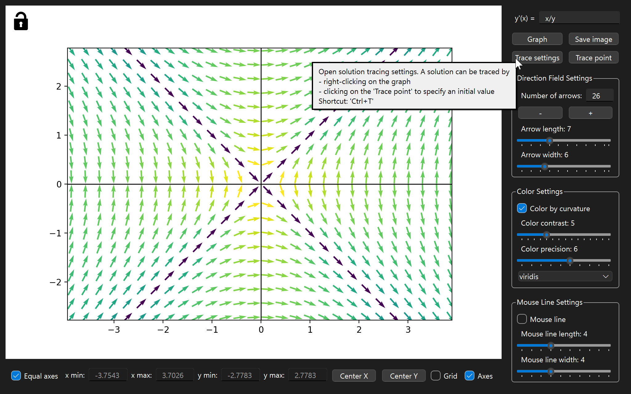
- Entering the differential equation
- Movement in the figure
- Exporting the figure
- Direction Field Settings
- Color Settings
- Mouse line settings
- Tracing solution curves
- Changing the limits of the coordinate axes
-
The differential equation must be syntactically correct. For example, you can't write
2xinstead of2*x. Use**for exponentiation. The available functions are-
sin,cos,tan,asin,acos,atan -
sinh,cosh,tanh,asinh,acosh,atanh, -
exp,ln=log,log2,log10 -
abs,sign,floor,ceil,min,max -
sqrt,pow - constants
piande - Use
powwhen raising to a fractional power. For example$x^{3/2}$ should be written aspow(x, 3/2).x**(3/2)will not work.
-
-
Confirm the differential equation by pressing the
Enterkey or by clicking theGraphbutton. -
In fact any valid python oneliner which returns a number can be used. You can for example do things like
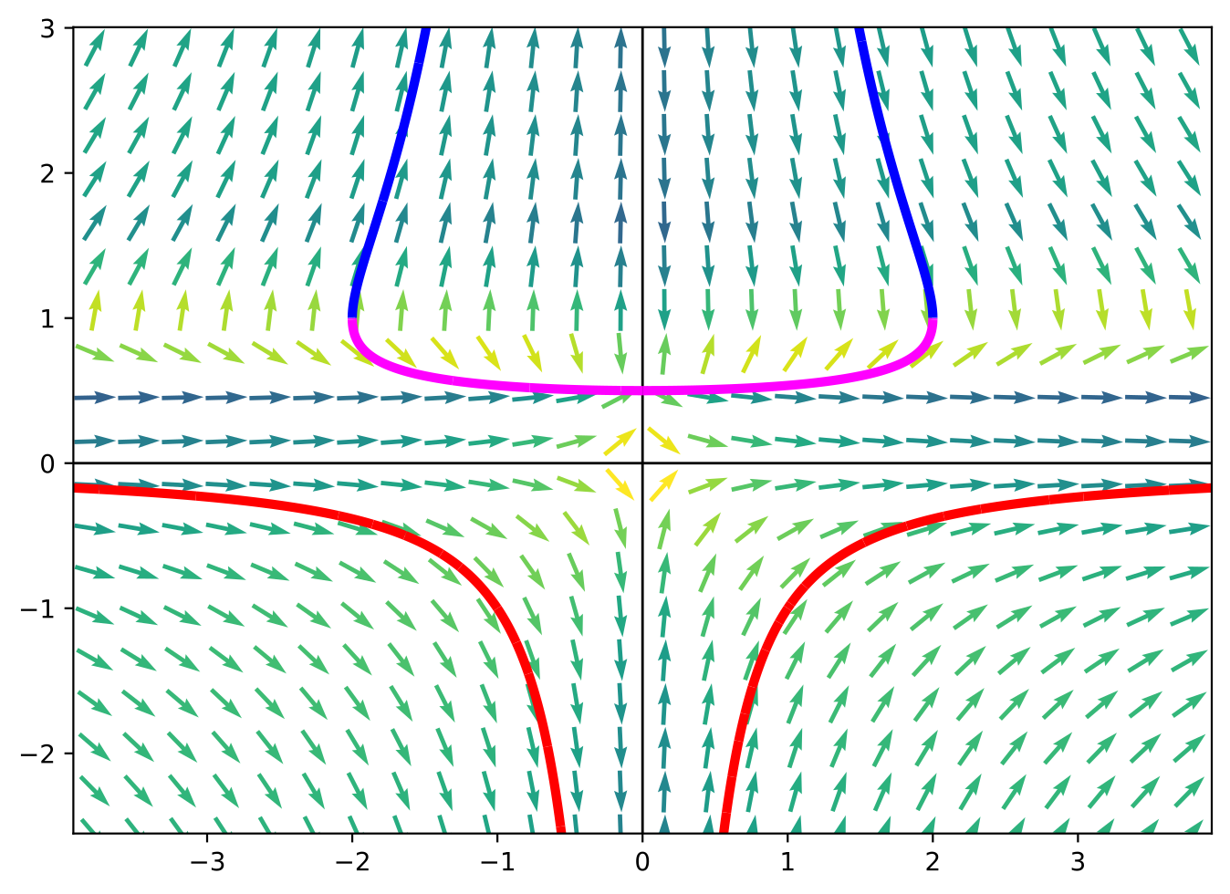
y' = x/(0 if abs(x-y)<1 else y)which produces the following plot: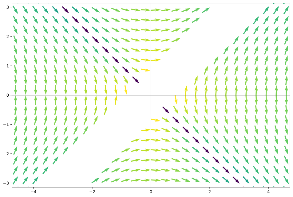
- The graph can be moved by left-clicking and dragging
- You can also zoom in and out using the scroll wheel
- It is possible to lock the canvas and disable movement by clicking on the
Lockbutton. You might want to do this when tracing a lot of curves to prevent accidental movement and therefore erasing the curves
- The figure can be exported as a
.png,.svgor.pdffile by clicking theSave imagebutton or by pressingCtrl+S
- The number of arrows can by changed either by entering a number or by clicking the
+and-buttons which change the value by 5 - It is also possible to change the width and the length of the arrows
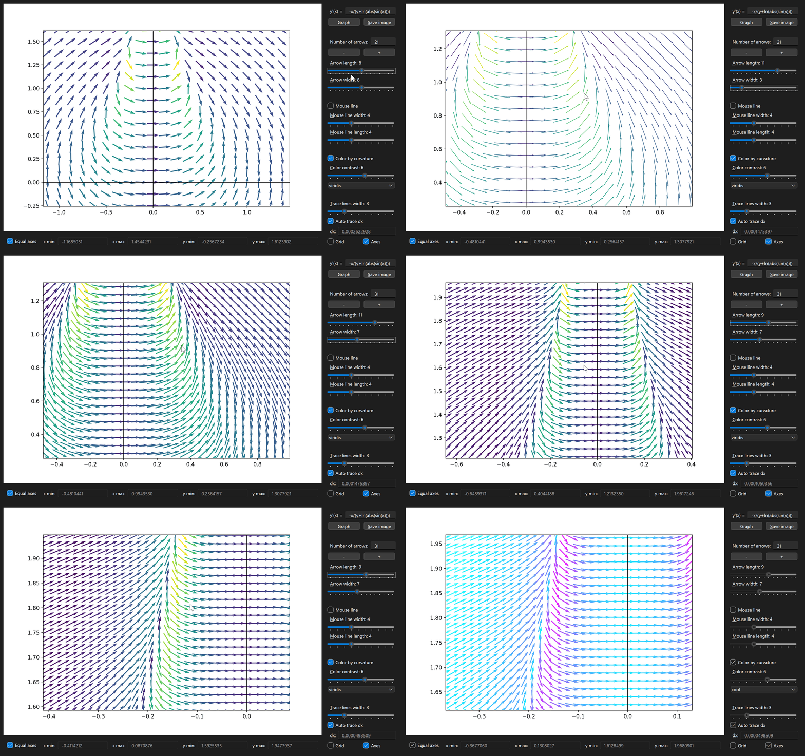
- The arrows can be colored based on the curvature of the solution curve at the point where the arrow is tangent to the curve
- This is on by default, but can be toggled off using the
Color by curvaturecheckbox - There are many different color schemes to choose from, I encourage you to try them all
- Some color schemes are showcased in the gallery
- By changing the
Color contrastslider, you can change the contrast of the colors. Lower values mean that even slight changes in curvature will result in a change in color.
Color precision
-
By changing the
Color precisionslider, you can influence the size of$dx$ used to calculate the curvature. Higher precision means smaller$dx$ which means more accurate curvature. Most of the time you won't need to change this value. There are two situations where you might want to change it:- If there are weird artifacts in the coloring, try increasing the precision. This might happen when dividing by zero or when infinities are involved
Precision=3 Precision=8 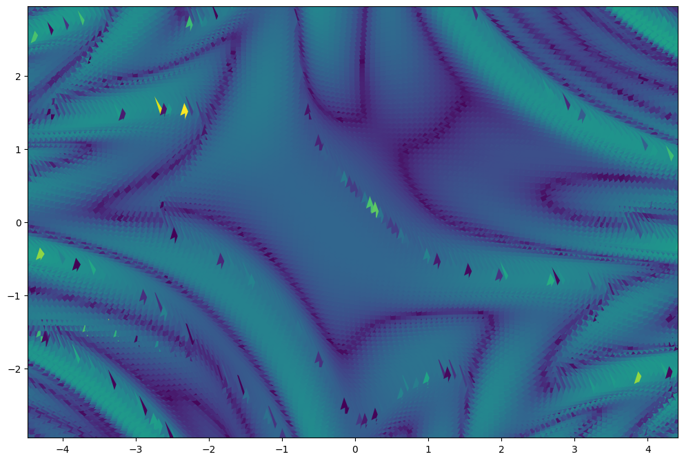
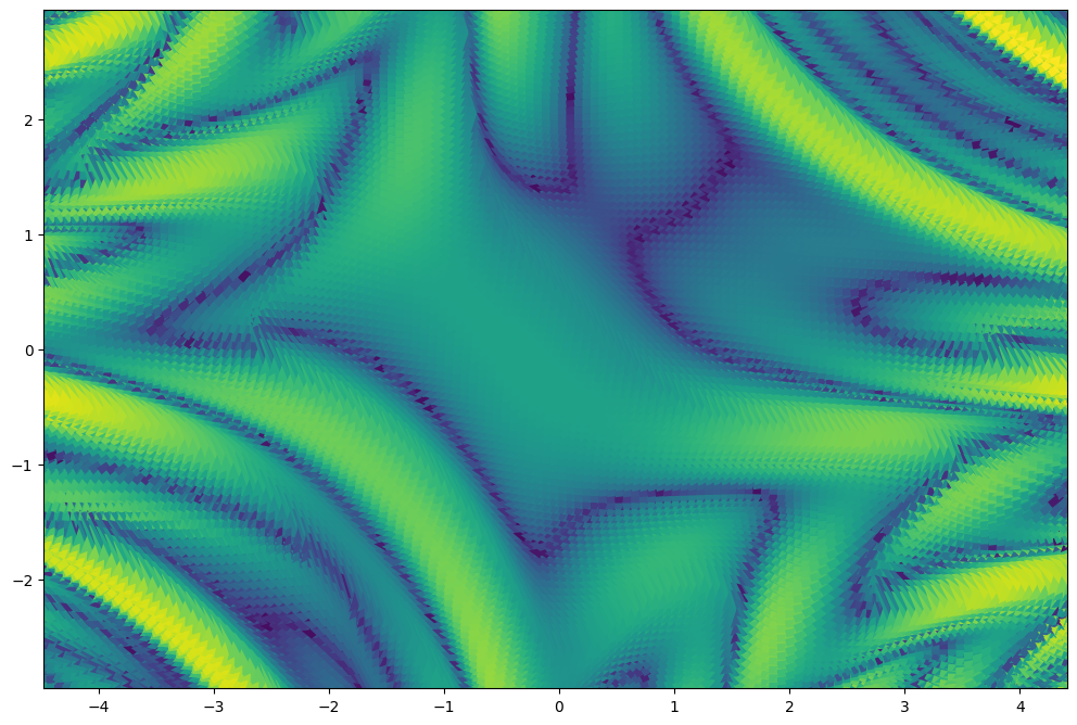
- If there are some parts of the curve that have really high curvature, they might overpower the rest of the colors. In this case, you can decrease the precision.
Precision=5 Precision=2 

- To draw a tangent line at the cursor's position, toggle
Mouse lineon. It is off by default - You can change the width and length of this line
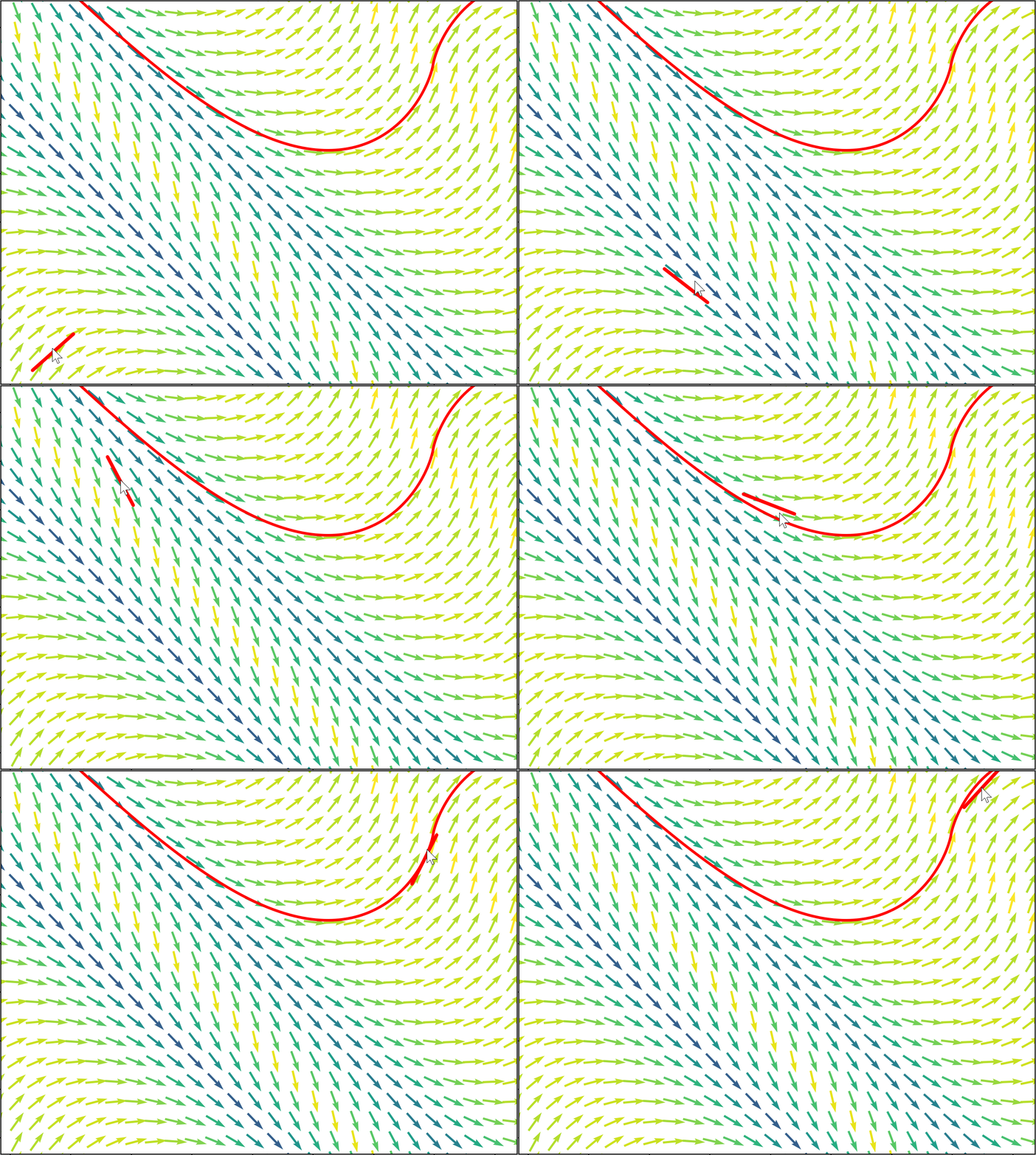
- To trace a solution curve, right-click and a solution passing through that point will be drawn
- If you need to specify the initial condition exactly, you can do so by clicking the
Trace pointbutton and entering the$x$ and$y$ coordinates of the point - Erase all drawn curves by moving, left-clicking, changing the parameters of the plot or by pressing
Ctrl+R(like in reset) - If the tracing is taking too long, the Stop button will appear in the top right corner of the plot. You can stop the tracing by clicking it or by pressing the
ESCkey
Trace Settings
-
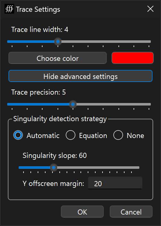
The
Trace settingsdialog allows you to change- the width and color of the curves
- the strategy used for detecting and dealing with singularities
-
Singularity is a point where the slope of the function goes to infinity. The function itself can either
- go to infinity, e.g.
$y = 1/x$ has a singularity at$x=0$ - abruptly stop, e.g.
$y = \sqrt{1-x^2}$ has singularities at$x=\pm1$
- go to infinity, e.g.
-
Trace precisionslider- Trace precision directly affects the step size used to trace the solution curve
- This affects both Automatic and Equational detection
- Higher precision means exponentially smaller step size and exponentially higher calculation time
- It is highly advised to use equational singularity detection over increasing precision
- Increase precision only if a singularity is not being detected correctly
-
Automatic detection (defulat)
- Works well in most cases, uses the slope of the function to detect singularities
- If the slope of the function exceeds a certain threshold, the algorithm will dramatically decrease the step size and be more cautious. This also means an increase in computation time
- You can change the slope threshold by moving the
Singularity slopeslider - A solution curve might go off the screen in the y-direction. It might but also might not come back. The
Y offsreen margindetermines for how long the calculation continues after the curve goes off the screen.- Lets say that the height of the plot is 4, the y-center being 0 and the
Y offsreen marginbeing 20. The curve will be cut off once it reaches$y=4/2+20\cdot 4=82$ or$y=-82$ . - Basically, the
Y offsreen marginis the number of times the height of the plot that the curve can go off the screen. - You can increase this value if the curve is not coming back but you know it should.
- Lets say that the height of the plot is 4, the y-center being 0 and the
-
Equational detection
- Faster, more reliable and more accurate than automatic detection
- You have to enter an equation that gives the singularities of the function
- This also means that if you enter the wrong equation, the tracing will not work properly
- The equation should be in the form of
$f(x, y) = 0$ - Examples:
$y' = x/y \quad\longrightarrow\quad y=0$ -
$y' = (x+y)/\ln(\mathop{\text{abs}}(x)) \quad\longrightarrow\quad \ln(\mathop{\text{abs}}(x))=0$ or$\mathop{\text{abs}}(x)-1=0$ $y' = y\ln(x) \quad\longrightarrow\quad x=0$ $y' = \tan(x) \quad\longrightarrow\quad \cos(x)=0$
- What if there are multiple singularities? Just multiply them together!
$y' = y/x + \ln(\sin(y)) \quad\longrightarrow\quad x\sin(y)=0$
-
No detection
- Chose this if you know that the function doesn't have any singularities
- It will be faster than the other two methods, because it won't have to check for singularities
- By default
Equal axesis toggled, but you can untoggle it to change the limits independently - You can't change limits manually while
Equal axesis toggled - Grid lines can be toggled on and off - they are off by default
- The coordinate axes can be toggled on and off - they are on by default
- The
Center XandCenter Ybuttons center the plot on the x-axis and y-axis respectively