Web_Example

First Example: Web Interface

This page walks through a complete solve in the web interface. The example finds the smallest interval that contains a set of sampled points and certifies how likely a new point is to fall outside it. You will:

1. enter the problem by hand in the matrix editors (Route A), or load it in one step from a program file (Route B);
2. upload the scenario data and solve;
3. read every number in the results;
4. optionally, run a parameter sweep and look at the graph it produces.

Use the hosted app at https://scen-opt.woodingben.com or a local copy (see Local Install). The steps and numbers on this page were checked against the current code with the default solver, CLARABEL.

The problem

We have $N = 100$ points $\delta_1,\ldots,\delta_{100}$ sampled from $[0, 1]$. We want the shortest interval $[o - w,\ o + w]$ that contains all of them, with centre $o$ and half-width $w$. The decision variable is

$$x = \begin{bmatrix} o \\ w \end{bmatrix} \in \mathbb{R}^2 .$$

Point $\delta_i$ lies in the interval when $o - w \le \delta_i \le o + w$. This is the same as two linear inequalities:

$$-o - w + \delta_i \le 0, \qquad o - w - \delta_i \le 0 .$$

In Scen-Opt's LP form, $A(\delta)\ x + b(\delta) \le 0$, this gives

$$c = \begin{bmatrix} 0 \\ 1 \end{bmatrix}, \qquad A(\delta) = \begin{bmatrix} -1 & -1 \\ 1 & -1 \end{bmatrix}, \qquad b(\delta) = \begin{bmatrix} \delta \\ -\delta \end{bmatrix} .$$

The problem is a robust LP: minimize $c^\top x = w$ subject to $A(\delta_i)\ x + b(\delta_i) \le 0$ for $i = 1,\ldots,N$. It has no regularization ($\tau = 0$), no relaxation ($\rho = 0$) and no hard constraints. The sizes are:

Size	Value	Meaning
$d$	2	decision variables
$\mathfrak{m}$	2	rows of $A(\delta)$ and $b(\delta)$
$\mathfrak{n}$	0	rows of $G$ and $h$ (none)
$q$	1	uncertainty dimension: each scenario is a single number

The risk of a solution $x$ is the probability that a new point, drawn from the same unknown distribution as the data, falls outside the interval. We bound the risk with confidence $1 - \beta$, using $\beta = 10^{-6}$.

Get the files

The example is the LP_half_width_2d benchmark. Its data folder is benchmarks/LP_half_width_2d/data/. Download two files:

• scenarios.csv: the 100 scenarios, one number per line, with no header.
• program_symbolic.json: the whole problem definition. You need it for Route B only.

In symbolic mode, a scenario file has one row per scenario and one column per component of $\delta$. In a CSV file, the columns are separated by commas.

The interface at a glance

Element	Where	What it does
LP / QP / SDP tabs	top left	Choose the program class.
Upload Program	top right	Load a complete problem from a JSON or MAT file (Route B).
Symbolic / Numeric switch	top of the program card	Choose how the scenario-dependent matrices are given. This example uses Symbolic.
Select Option	program card	Choose the formulation: Robust, Regularization, Relaxation, or Regularization + Relaxation.
Formula	program card	Shows the program for the chosen option. Its symbols match the names on the input buttons.
Dimension fields $d$, $\mathfrak{m}$, $\mathfrak{n}$	below the formula	Set the problem sizes. Changing a size reshapes the matrices you have already entered: it pads with zeros or cuts off entries.
Edit $c$, Edit $A(\delta)$, Edit $b(\delta)$, Edit $G$, Edit $h$	program card	Open a matrix editor.
$\tau$, $\bar{x}$, $p$, $\rho$ fields	program card	Appear only when the chosen option uses them.
Confidence $1-\beta$ where $\beta$	lower left	Enter $\beta$ here.
Solver	lower left	Solvers installed on the server that suit the active program type.
Scenarios	lower right	Upload the scenario data file.
Solve	lower right	Validate the inputs and run the solve.
Result	bottom	Results table, graphs and downloads.

Most inputs have a ? icon. Hover over it to see a short explanation.

Each matrix editor has:

• a grid with one input box per entry, sized from the dimension fields;
• an Or paste JSON content box;
• an Input Format Reference section.

The editor checks entries as you type. If the paste box is not empty when you press Save, its content replaces the grid.

Route A: enter the matrices in the editors

1. Open the app. The LP tab, the Symbolic mode and the Robust option are already selected. The formula reads $\min_x\ c^\top x$ subject to $A(\delta_i)\ x + b(\delta_i) \le 0$ and $Gx + h \le 0$.

2. Set the dimensions:

   • leave $d$ at 2;
   • change $\mathfrak{m}$ from 1 to 2;
   • change $\mathfrak{n}$ from 1 to 0.

   With $\mathfrak{n} = 0$, the Edit $G$ and Edit $h$ buttons are greyed out, because the problem has no hard constraints.

3. Click Edit $c$. In the 2×1 grid, enter 0 and 1, then press Save.

4. Click Edit $A(\delta)$. In the 2×2 grid, enter -1, -1 in the first row and 1, -1 in the second row. Press Save.

5. Click Edit $b(\delta)$. In the 2×1 grid, enter delta[0] and -delta[0], then press Save.

   delta[0] is the first component of $\delta$, which is the first column of the scenario file. Here $\delta$ has only one component.

6. In Confidence $1-\beta$ where $\beta$, enter 1e-6. This field takes $\beta$ itself, not $1-\beta$. If you leave it empty, $\beta$ is taken as 0 and the upper risk bound becomes the trivial value 1.

7. Leave Solver at CLARABEL, the first entry in the list.

8. Under Scenarios, click Choose File and select scenarios.csv.

9. Press Solve.

Pasting JSON instead of typing. In step 5, for example, you can paste [["delta[0]"], ["-delta[0]"]] into the editor's paste box instead of filling the grid. Write every entry as a quoted string, e.g. [["0"], ["1"]] for $c$. The current server rejects unquoted numbers such as [[0], [1]]:

• in $c$, $G$, $h$ or $Q$, they cause an Internal Server Error after Solve;
• in $A(\delta)$ or $b(\delta)$, the Error row shows compile() arg 1 must be a string, bytes or AST object.

Checks before solving. If an input is missing or has the wrong shape, Scen-Opt does not send the problem to the server. Instead, a red message appears above Solve, for example A(δ) is 1×2 but expected 2×2. or No scenarios file uploaded. …. Fix the input and press Solve again.

Route B: upload the whole program

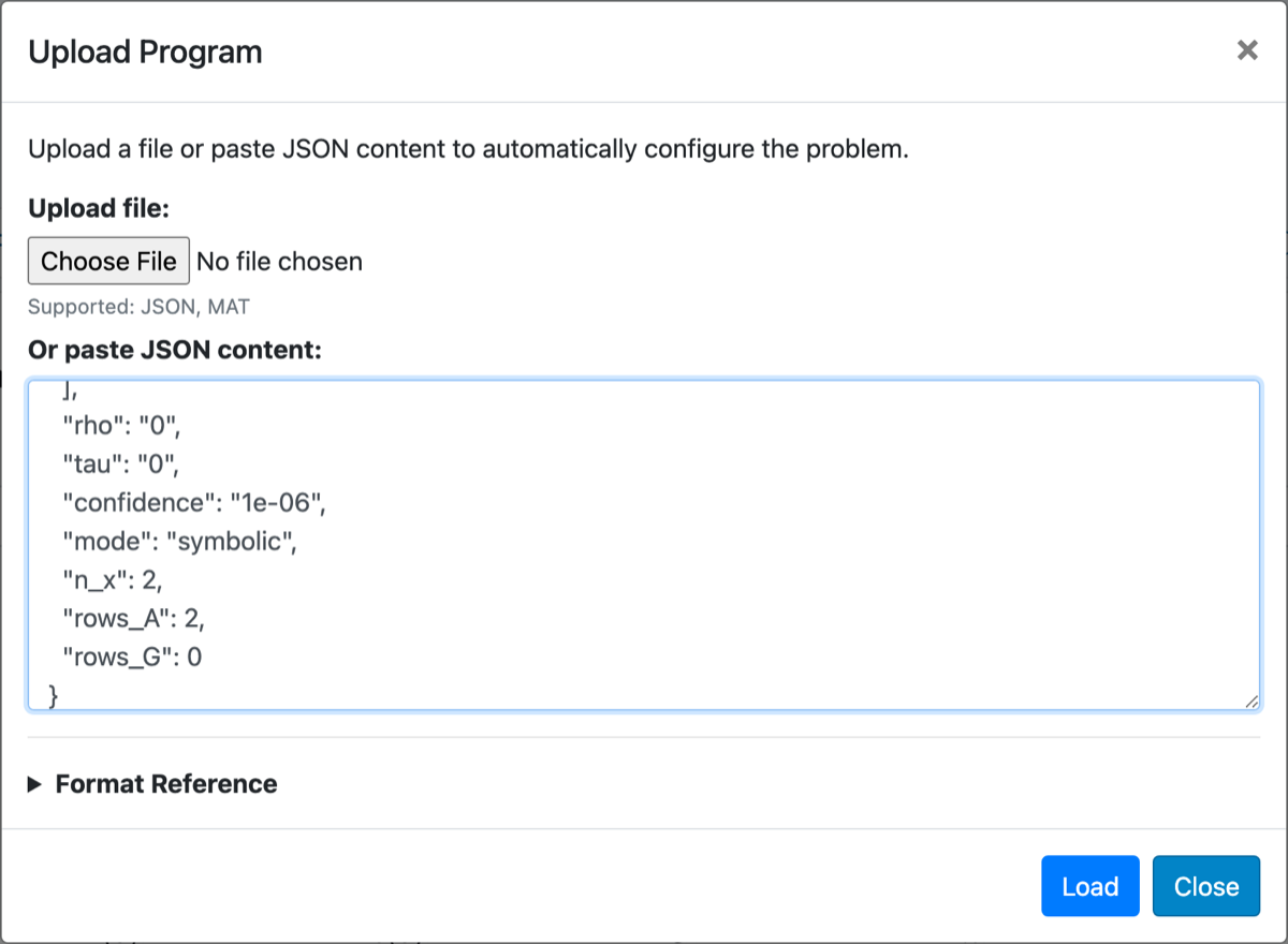
1. Open the app and click Upload Program (top right).

2. Give the program in one of two ways:

   • under Upload file, choose program_symbolic.json; or
   • paste the file's text into Or paste JSON content.

   If you do both, the file is used.

3. Click Load. A message confirms: LP problem loaded successfully. Upload scenarios and press Solve.

   The page is now set up exactly as at the end of step 6 of Route A:

   • LP tab, Symbolic mode, Robust option;
   • $d = 2$, $\mathfrak{m} = 2$, $\mathfrak{n} = 0$;
   • $c$, $A(\delta)$ and $b(\delta)$ filled in;
   • $\beta$ = 1e-06.

   Loading a program clears, on every tab, the matrices and the $\tau$, $\rho$, $p$ and $\bar{x}$ fields, and removes any earlier result. The $\beta$ field keeps its old value unless the file sets confidence.

4. Under Scenarios, choose scenarios.csv. The program file does not contain the scenarios; you always upload them separately.

5. Leave the solver at CLARABEL and press Solve.

The program file contains the following (reformatted here; the key order does not matter):

{
  "type": "LP",
  "mode": "symbolic",
  "n_x": 2,
  "rows_A": 2,
  "rows_G": 0,
  "c":   [["0"], ["1"]],
  "A_d": [["-1", "-1"], ["1", "-1"]],
  "b_d": [["delta[0]"], ["-delta[0]"]],
  "rho": "0",
  "tau": "0",
  "confidence": "1e-06"
}

The meaning of every key is given in Program file reference below.

Variant: numeric mode

The same folder has a numeric version of the problem, for use when you cannot write the constraints as formulas.

• Program file. program_numeric.json sets "mode": "numeric" and contains no A_d or b_d.
• Scenario file. Each row of scenarios_numeric.csv holds one scenario's evaluated constraint data. It contains $A_i$ flattened row by row, followed by $b_i$: $[\ A_{11}, A_{12}, A_{21}, A_{22}, b_1, b_2\ ] = [-1, -1, 1, -1, \delta_i, -\delta_i]$. That is $\mathfrak{m} d + \mathfrak{m} = 6$ numbers per row.

To use it:

1. Load program_numeric.json with Upload Program. The switch moves to Numeric, and the $A(\delta)$ and $b(\delta)$ buttons disappear.
2. Upload scenarios_numeric.csv and press Solve.

The results are the same as in symbolic mode.

Results

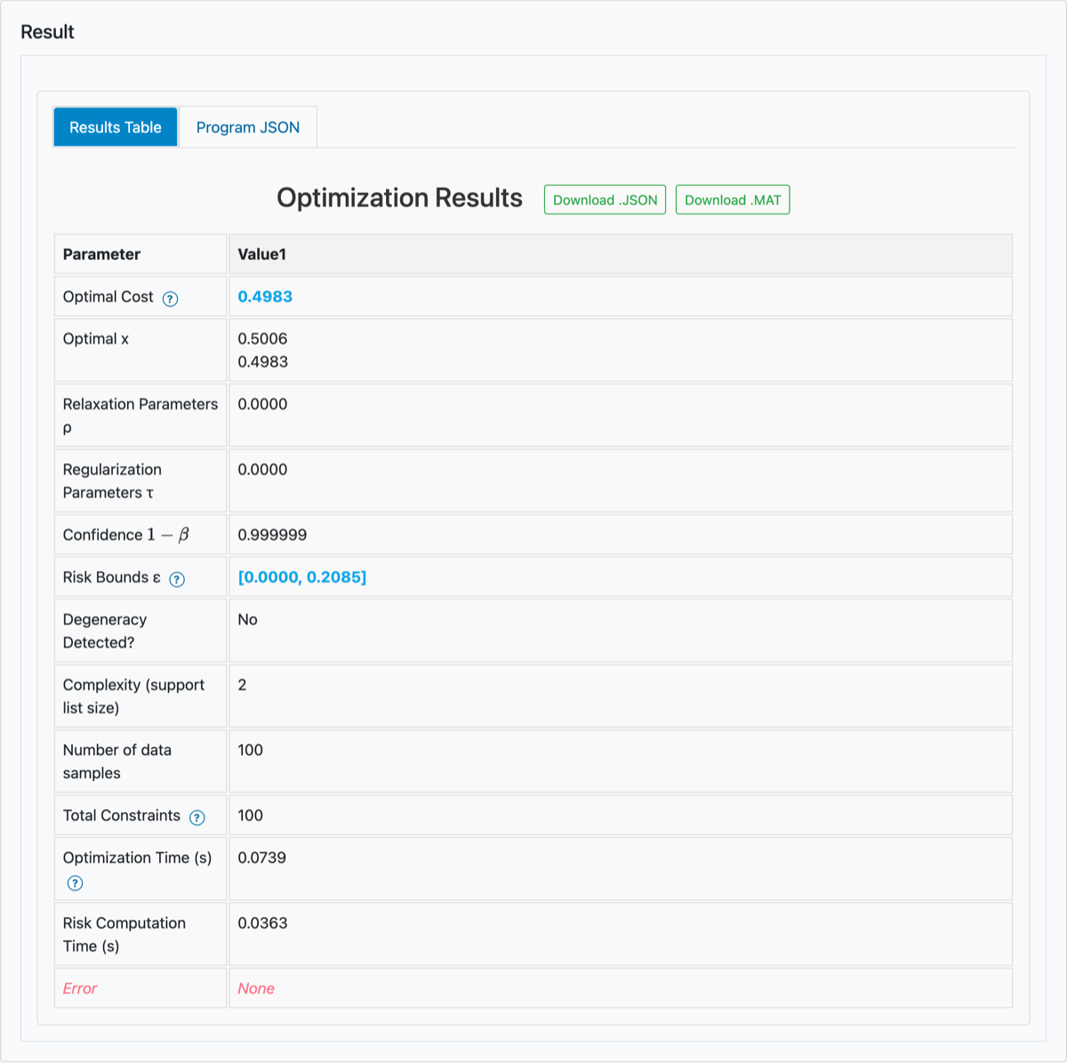
Both routes give the same Results Table. The table rounds numbers for display; the downloads keep full precision. Times vary from run to run.

Row	Shown	Meaning
Optimal Cost	0.4983	$c^\top x^\ast = w^\ast$. For LPs this is $c^\top x^\ast$; for QPs and SDPs it is $c^\top x^\ast + \tfrac12 x^{\ast\top} Q x^\ast$. The $\tau$ and $\rho$ penalty terms are never included.
Optimal x	0.5006, 0.4983	$x^\ast = [o^\ast,\ w^\ast]$: centre and half-width.
Relaxation Parameters ρ	0.0000	The $\rho$ used for this solve.
Regularization Parameters τ	0.0000	The $\tau$ used for this solve.
Confidence $1-\beta$	1.0000	$1 - 10^{-6} = 0.999999$, rounded to four decimals.
Risk Bounds ε	[0.0000, 0.2085]	$[\varepsilon_L, \varepsilon_U]$.
Degeneracy Detected?	No	Whether the lower bound is certified (see below).
Complexity (support list size)	2	$k$.
Number of data samples	100	$N$.
Total Constraints	100	Number of scenario constraints: one per scenario, here each a 2-row block. Hard constraints are not counted.
Optimization Time (s)	varies (well under 1 s here)	Time for the solve, including the support-list computation.
Risk Computation Time (s)	varies (well under 1 s here)	Time to compute the risk bounds.
Error	None	Error message from the solver, if any.

At full precision, $x^\ast = [0.5006347,\ 0.4983100]$ and $\varepsilon_U = 0.2085241$.

What the numbers mean

• The interval. $[o^\ast - w^\ast,\ o^\ast + w^\ast] = [0.0023,\ 0.9989]$. Its ends are the smallest and the largest data point, which are on lines 90 and 95 of scenarios.csv.

• Complexity $k = 2$. These two points form the support list. Removing either one would shrink the interval; removing any other point changes nothing.

• Risk bounds. With confidence at least $1 - 10^{-6}$, the probability that a new point from the same distribution falls outside the interval is between 0 and 0.2085. Nothing is assumed about the distribution.

  • The upper bound $\varepsilon_U$ holds for every solution.
  • The lower bound $\varepsilon_L$ holds only for non-degenerate problems. Here Degeneracy Detected? is No, so both bounds apply. When the flag is Yes, the table still shows a number for $\varepsilon_L$, but you should rely only on $\varepsilon_U$.

  See Scenario Theory for the theorems.

• The bounds depend only on $k$, $N$ and $\beta$. For $N = 100$ and $\beta = 10^{-6}$:

  $k$	0	1	2	3
  $[\varepsilon_L, \varepsilon_U]$	[0, 0.1586]	[0, 0.1858]	[0, 0.2085]	[0, 0.2289]

  A solution supported by fewer scenarios receives a tighter certificate.

The benchmark's own figure shows the same results:

• (a) the interval and its two support scenarios (the figure calls the half-width $h$);
• (b) the bounds as functions of $k$;
• (c) a histogram of the data.

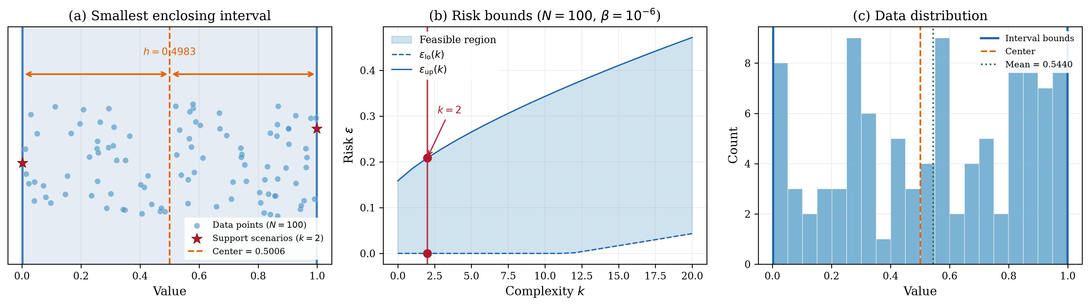
Solver accuracy matters for $k$. Scen-Opt finds the support list by re-solving the problem without some of the scenarios and comparing optimal values. This needs accurate solutions. If you select SCS for this example, the result is $k = 99$ with Degeneracy Detected? Yes, and the bounds become [0.7926, 1]. Use an accurate interior-point solver such as CLARABEL or MOSEK. If $k$ looks too large, or degeneracy is flagged unexpectedly, try another solver.

Result tabs and downloads

Tab	When shown	Content
Results Table	always	The table above, with Download .JSON and Download .MAT buttons.
ρ Graph	options Relaxation and Regularization + Relaxation	Risk bounds and cost plotted against $\rho$.
τ Graph	options Regularization and Regularization + Relaxation	Risk bounds and cost plotted against $\tau$.
Program JSON	always	The problem as an Upload Program file, with a Download Program (.JSON) button. Upload this file later to restore the same set-up.

For the robust example, only Results Table and Program JSON appear.

Download .JSON saves results.json; Download .MAT saves results.mat, which the server generates. Both files contain the keys below. Each key holds a list with one entry per $(\tau, \rho)$ pair, except conf and n_attempts.

Key	Content
optimal_x	optimal $x$
optimal_s	slacks $\zeta_i$
optimal_cost	optimal cost
num_deltas	$N$
tot_con	number of scenario constraints
active_con	$k$
risk	$[\varepsilon_L, \varepsilon_U]$
conf	the reported overall confidence
rho_, tau_	the parameter values
degeneracy	degeneracy flag
errorcode	error message, or None
solve_time, risk_time	times in seconds
n_attempts	number of solves

Optional: a relaxation sweep

With relaxation, the interval may leave some points outside. Each unit of violation costs $\rho$ in the objective. Lists of $\rho$ values show the trade-off between cost and risk.

1. After the robust solve, change Select Option to Relaxation.
   • The formula changes to $\min_{x,\ \zeta_i \ge 0}\ c^\top x + \rho \sum_i \zeta_i$ subject to $A(\delta_i)\ x + b(\delta_i) \le \zeta_i$.
   • A $\rho \ge 0$ field appears.
   • Changing the option clears the $\tau$, $\rho$, $p$ and $\bar{x}$ fields.
2. In the $\rho$ field, enter 0.07,0.15,0.3,1. A counter n_ρ = 4 appears above the confidence field, and its label changes to "Confidence $1 - \beta \cdot n_\rho$ where $\beta$".
3. Press Solve. Scen-Opt solves four programs, one per value of $\rho$, and the table gets one column per value:

$\rho$	0.07	0.15	0.3	1
Optimal cost $w^\ast$	0.4517	0.4779	0.4923	0.4983
Points outside the interval	14	6	2	0
Complexity $k$	16	8	4	2
Risk bounds	[0.0221, 0.4234]	[0, 0.3137]	[0, 0.2476]	[0, 0.2085]
Degeneracy detected	No	No	No	No

The point counts come from the Optimal ζ row, which now appears in the table. Entries of order $10^{-12}$ in that row are solver round-off, not violations.

Reading the table:

• A smaller $\rho$ makes violations cheaper. The interval gets narrower and leaves more points outside.
• The support list then contains the violated points plus the two boundary points, so $k$ grows. The risk certificate gets weaker as $k$ grows.
• At $\rho = 1$, no point is outside, and the result equals the robust solution.

Confidence. The certificate now covers all four solves together (a union bound), so the table reports $1 - 4\beta = 0.999996$ (displayed as 1.0000).

Choice of values. The values $0.07, 0.15, 0.3$ were chosen to avoid ties. For $\rho = 0.5/n$ with integer $n$ (e.g. 0.5, 0.25, 0.1), several intervals are optimal, because moving one end of the interval over a stretch of the line does not change the objective.

The ρ Graph tab now appears. It plots the lower bound (green), the upper bound (blue) and the cost (black) against $\rho$. When several $\tau$ values are also swept, a Select τ menu chooses which slice to show. See In-built Graphics.

Program file reference

The Upload Program dialog reads the keys below. Its Format Reference section lists them for each program type.

Key	Needed	Meaning
type	always	"LP", "QP" or "SDP". Selects the tab.
mode	optional	"symbolic" (default) or "numeric".
option	optional	"robust", "regularization", "relaxation" or "regularization-relaxation". See the note below the table.
n_x	optional	$d$, the number of decision variables. For LP/QP the dialog takes $d$ from the number of rows of c, so n_x must agree with it.
rows_A	numeric mode	$\mathfrak{m}$, the rows of $A(\delta)$ and $b(\delta)$. It is taken from A_d when A_d is given, so you need it only in numeric mode.
rows_G	optional	$\mathfrak{n}$, the rows of $G$ and $h$. It is taken from G when G is given. The value 0 means no hard constraints.
c	always	Cost vector, $d \times 1$.
A_d	symbolic LP/QP	$A(\delta)$, $\mathfrak{m} \times d$; entries may contain delta[k].
b_d	symbolic LP/QP	$b(\delta)$, $\mathfrak{m} \times 1$; entries may contain delta[k].
G, h	optional	Hard constraints $Gx + h \le 0$: $\mathfrak{n} \times d$ and $\mathfrak{n} \times 1$, numbers only. Give both or neither.
Q	QP	$d \times d$, symmetric and positive semidefinite. Optional for SDP.
rho	for relaxation	$\rho \ge 0$. A single value or a comma-separated list, e.g. "0.07,0.15,0.3,1".
tau	for regularization	$\tau \ge 0$. A single value or a comma-separated list.
confidence	set it	$\beta$ itself, e.g. "1e-06", not $1-\beta$.
p	optional	Norm order for regularization: a number $\ge 1$, "inf" or "fro". Default 2.
x_ref	optional	Regularization reference point $\bar{x}$, $d \times 1$.
F_d, E, lmi_size, lmi_e_size	SDP	See Semidefinite Programs.

How option is inferred. If option is missing, a rho above 0 switches on relaxation and a tau above 0 switches on regularization. The inference reads only the first number of a list. For a sweep that starts at 0, such as "0,0.5,1", set option explicitly.

Rules for entries

• Every matrix and vector is a 2-D array of rows. A vector is a column: "c": [["0"], ["1"]].
• Write every entry as a quoted string, as the benchmark files do: "0", "-1", "delta[0]". The current server rejects unquoted numbers. In c, G, h or Q they cause an Internal Server Error when you press Solve; in A_d or b_d the Error row reports the failure.
• delta[k] is 0-indexed. delta[0] is the first column of the scenario file, and delta[q-1] is the last.
• Allowed expression syntax in A_d, b_d (and F_d):
  • numbers;
  • the operators + - * / // % ** and parentheses;
  • delta[k];
  • functions and constants from Python's math module, written with the math. prefix, e.g. math.sin(delta[1]), math.exp(delta[0]), math.pi. A bare sin(...) is rejected.
• c, G, h, Q and x_ref hold numbers only (still written as quoted strings). They cannot contain delta.
• Unused optional fields can simply be omitted, as in the benchmark program files.
• MAT files use the same variable names. Store matrix variables as cell arrays of strings, e.g. c = {'0'; '1'} and b_d = {'delta[0]'; '-delta[0]'}. Numeric arrays currently cause the same server error as unquoted numbers in JSON. Scalars such as rho = 0 may be plain numbers.

Troubleshooting

Symptom	Cause and fix
Red message above Solve	An input is missing or has a shape that does not match $d$, $\mathfrak{m}$, $\mathfrak{n}$, or no scenario file has been chosen. The message names the problem.
Server error (500): Internal Server Error	An entry was given as an unquoted number (JSON paste box, program file, or MAT numeric array), or the scenario file contains something that is not a number, such as a header row.
The Error row shows a message	The solver failed for that column, e.g. MOSEK license cannot be located or is incorrect. (see Local Install). Try another solver or check the inputs.
Upper risk bound is 1 and the confidence shows 1.0000	The $\beta$ field was empty, so $\beta = 0$. Enter a value such as 1e-6.
Large $k$ or unexpected degeneracy	Possibly an inaccurate solver (see the SCS note above). Try CLARABEL or MOSEK.
Problem loaded with the wrong formulation	Add an explicit option key to the program file.

Next steps

• First Example: Python Calls: solve the same problem from Python.
• Linear Programs: all LP options, including hard constraints and numeric mode.
• In-built Graphics: the ρ and τ graphs in detail.
• Scenario Theory: where the risk bounds come from.
• The other benchmarks: each of the twelve case studies in benchmarks/ (listed in the repository README) has a data/ folder with the pairs program_symbolic.json + scenarios.csv and program_numeric.json + scenarios_numeric.csv. You can load them in the same way.