With ongoing advancements in deep learning-based computer vision models, object detection applications are simpler to build than ever before. Object detection is an advancement to image classification. In general, Image classification involves categorizing an image by assigning a label to it whereas, object detection involves classifying the object inside the images by assigning a label to them. (Hulstaert, 2018). An example of object detection is as given below

The TensorFlow Models GitHub repository provides an excellent object detection API. This object detection API by Google makes it extremely easy to train your own object detection model for a large variety of different applications. In this assignment, Tensorflow Object Detection API was trained and validated for detection of Formula 1 cars. will have the detailed steps for building a Formula 1 Object detection model using TensorFlow’s API.
Steps followed to build a tensorflow model
-
Installation of Tensorflow and other related components
-
Gather Datasets
-
Annotating gathered images
-
Generate Tensorflow Training Record
-
Choose the model
-
Configure and Train the model.
-
Export the frozen inference graph
-
Validate your model
Anaconda is a useful tool, to setup any tool/library like Tensorflow when working with Python. Hence, it is good to have anaconda installed.
Tensorflow can be setup in GPU or CPU. It is easy to install Tensorflow on a CPU, but the performance will be low as it runs computationally heavy Machine learning Algorithms. Alternatively, if the machine has CUDA enabled Nvidia graphics card, the Tensorflow GPU speeds up while training the model (TensorFlow, 2019) . To install TensorFlow on a GPU, the hardware pre-requisite is NVIDIA GPU card with CUDA Compute Capability 3.5 or higher and the software pre-requisites are as follows:
· NVIDIA GPU drivers —CUDA 10.0 requires 410.x or higher.
· CUDA Toolkit —TensorFlow supports CUDA 10.0 (TensorFlow >= 1.13.0)
· CUPTI ships with the CUDA Toolkit.
· cuDNN SDK (>= 7.4.1)
Apart from these, TensorRT 5.0 installation will improve the latency and throughput for inference on some models. However, it is optional (TensorFlow, 2019).
Firstly, create a new Conda virtual environment by using the following command in the command prompt/ Anaconda prompt
C:> conda create -n tensorflow1
Then, activate the environment by using the following command
**C:\>** `activate tensorflow1`
To install tensorflow in this environment use the following command
C:\> pip install tensorflow-gpu Or C:\> pip install tensorflow (For CPU versions)
Once done verify installation of Tensorflow by starting an interpreter session as below

Fig 1. Screenshot of Tensorflow installation verification
If there are no errors then, Tensorflow is installed successfully. (Vladimirov, n.d.)
Even if the machine has NVIDIA drivers it should be CUDA enabled, else it cannot run on GPU. To verify whether the NVIDIA runs on CPU/GPU use the following code. (stackoverflow, n.d.)

Fig 2. Screenshot of Tensorflow using device list
In my case, Tensorflow can only run on CPU.
After installing Tensorflow, there are some packages which need to be installed before installing the models.
(tensorflow1) C:\> pip install pillow (tensorflow1) C:\> pip install lxml (tensorflow1) C:\> pip install Cython (tensorflow1) C:\> pip install contextlib2 (tensorflow1) C:\> pip install jupyter (tensorflow1) C:\> pip install matplotlib (tensorflow1) C:\> pip install pandas (tensorflow1) C:\> pip install opencv-python
After installing the packages, clone or download the Tensorflow Model repository from GitHub.
The Tensorflow repository is expected to maintain the below structure
TensorFlow1 ├─ models │ ├─ official │ ├─ research │ │ ├─Object_detection │ │ │ ├─images │ │ │ │ ├─Train │ │ │ │ ├─Test │ │ │ ├─Training │ │ │ │ ├─labelmap.pbtxt │ │ │ │ ├─Model_Config_file │ │ │ ├─Modelrepository │ ├─ samples │ └─ tutorials
Protobufs are used to configure model and training parameters. Before the framework can be used, the Protobuf libraries must be downloaded and compiled (Evan, 2019 )
(tensorflow1) C:\> conda install -c anaconda protobuf
This should be done by running the following command from the tensorflow/models/research/ object_detection directory:
protoc --python_out=. .\object_detection\protos\anchor_generator.proto .\object_detection\protos\argmax_matcher.proto .\object_detection\protos\bipartite_matcher.proto .\object_detection\protos\box_coder.proto .\object_detection\protos\box_predictor.proto .\object_detection\protos\eval.proto .\object_detection\protos\faster_rcnn.proto .\object_detection\protos\faster_rcnn_box_coder.proto .\object_detection\protos\grid_anchor_generator.proto .\object_detection\protos\hyperparams.proto .\object_detection\protos\image_resizer.proto .\object_detection\protos\input_reader.proto .\object_detection\protos\losses.proto .\object_detection\protos\matcher.proto .\object_detection\protos\mean_stddev_box_coder.proto .\object_detection\protos\model.proto .\object_detection\protos\optimizer.proto .\object_detection\protos\pipeline.proto .\object_detection\protos\post_processing.proto .\object_detection\protos\preprocessor.proto .\object_detection\protos\region_similarity_calculator.proto .\object_detection\protos\square_box_coder.proto .\object_detection\protos\ssd.proto .\object_detection\protos\ssd_anchor_generator.proto .\object_detection\protos\string_int_label_map.proto .\object_detection\protos\train.proto .\object_detection\protos\keypoint_box_coder.proto .\object_detection\protos\multiscale_anchor_generator.proto .\object_detection\protos\graph_rewriter.proto .\object_detection\protos\calibration.proto .\object_detection\protos\flexible_grid_anchor_generator.proto
Initially, tried the following command however, these commands don’t work on windows or Protbuf 3.5 or later (Vladimirov, n.d.)
<path-to-protoc> <path-to-tensorflow\models\research>\object_detection\protos\*.proto --python_out=.<path-to-protoc> <path-to-tensorflow\models\research>\object_detection\protos\*.proto --python_out=.
Initially, I faced issues in running the sample object detection pretrained model provided along with Tensorflow. As the environment variables were not set, the following error was shown. (Evan, 2019 )
Error: No module named 'deployment' or No module named 'nets'
The path “\TensorFlow\models\research\object_detection” must be added to Path in Environment variables->System variable section. In addition to this, add \research and \research\slim path
Also, it must be ensured if the commands from the \models\research directory: (Evan, 2019 ) are run.
setup.py build
setup.py install
These commands build and install the object_detection python package (Vladimirov, n.d.)
To ensure that the Tensorflow setup works, the object_detection_tutorial.ipynb script. (Evan, 2019 ) must be run.
By this the Tensorflow setup is verified that it is working properly.
For my data set, I decided to collect images of Formula 1 car from google image searches. As it was time consuming, I used the script to scrape images where I made sure that the images are ideal. (Kogan, n.d.). The script downloaded 308 images. I split 30% of all the data for testing (216 images for training, 92 images for testing).
For convenience, I resized all my images to 800 x 600 pixels to achieve uniformity and to facilitate putting the images into batches which help in speed gains. (Kathuria, n.d.).
The script needs to be saved in the parent directory of the images and be run like as below.
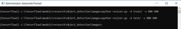
Fig4. Screenshot of running the script in command line
In order to train the object detection model, for each image, the image’s width, height is needed with their respective xmin, xmax, ymin, and ymax bounding box. LabelImg is an excellent open source free software that makes the labeling process much easier. It will save individual xml labels for each image, which will then be convert into a csv table for training. (Evan, 2019 )
However, there are semi-automation tools like FIAT (Fast Image Data Annotation Tool) and CVAT(Computer Vision Annotation Tool) for labelling the images. This might be useful in future. (christopher, n.d.) (Manovich, n.d.)
To Setup labelImg on windows requires ‘pyqt5’ package. The lableImg source from Github to a local directory is downloaded/cloned and navigated to that folder in Command prompt / Anaconda Prompt. Then the following commands are used.
conda install pyqt=5 [Or pip3 install labelImg] pyrcc5 -o libs/resources.py resources.qrc python labelImg.py
The labelImg will be opened, then navigated to Train and Test directory and a box is drawn around each object in each image similar to the screenshot below

Fig 5. Labeling the data using the LabelImg tool
After annotating the image, an xml file will be generated for each image once saved.
Before labeling, I changed all the images to single extension to avoid issues. To convert all the files to jpg I used the following command in command prompt from the directory
ren *. *.jpg
This converts all the files to .jpg extension. (stackoverflow, n.d.)
Now XML files needs to be converted to CSV files to convert to TFrecord. To convert xml to csv, I used an existing code from github (Tran, n.d.) Within the xml_to_csv script, I changed:
def main():
    image_path = os.path.join(os.getcwd(), 'annotations')
    xml_df = xml_to_csv(image_path)
    xml_df.to_csv('raccoon_labels.csv', index=None)
    print('Successfully converted xml to csv.')
To:
def main():
    for folder in ['train','test']:
        image_path = os.path.join(os.getcwd(), ('images/' + folder))
        xml_df = xml_to_csv(image_path)
        xml_df.to_csv(('images/' + folder + '_labels.csv'), index=None)
        print('Successfully converted xml to csv.')
After obtaining the.csv files, they are converted into TFRecords by running the generate_tfrecord.py script in research\object_detection. The generate_tfrecord.py script should have the label map, where each object is assigned an ID number. This same will be used when configuring the labelmap.pbtxt file. (Evan, 2019 )
def class_text_to_int(row_label): if row_label == 'F1': return 1 else: None
Once done, there will be 2 files generated , named, Train.record and Test.record which are generated using the following commands: (Evan, 2019 )
python generate_tfrecord.py --csv_input=images\train_labels.csv --image_dir=images\train --output_path=train.record python generate_tfrecord.py --csv_input=images\test_labels.csv --image_dir=images\test --output_path=test.record
When training models with TensorFlow using TFRecord, files help to optimize the data feed. (Francis, 2017)
Object detection is largely based on use of convolutional neural networks. Some of the most used models are Faster R-CNN, Multibox Single Shot Detector (SSD) and YOLO (You Only Look Once). Faster RCNN is an advancement of Region-based Convolutional Neural Network(R-CNN) or Fast R-CNN. The main aim of Faster R-CNN was to replace the slow selective search algorithm with a fast-neural net.
Multibox Single Shot Detector (SSD) differs from the R-CNN based approaches by not requiring a second stage per-proposal classification operation. This makes it fast enough for real-time detection applications.
YOLO (You Only Look Once) works on different principle than the models: it runs a single convolutional network on the whole input image (once) to predict bounding boxes with confidence scores for each class simultaneously. The advantage of the simplicity of the approach is that the YOLO model is fast (compared to Faster R-CNN and SSD) and it learns a general representation of the objects. This increases localization error rate (also, YOLO does poorly with images with new aspect ratios or small object flocked together) but reduces false positive rate.
Many modern object detection applications require real-time speed. Methods such as YOLO or SSD tends takes more time to train, whereas models such as Faster R-CNN achieve decent accuracy also takes less time to train. (pkulzc, 2019).

Screenshot of models pre-trained list
In the above screenshot the speed corresponds to the running speed of the model in milliseconds for larger images (e.g. 600x600. mAP is mean average precision which indicates how well the trained model performed on the COCO dataset.
The model speed depends for larger images (e.g. 600x600) . However, SSD works faster compared to more computational models such as R-CNN. Even on smaller images its performance is considerably lower . (Huang J, 2016). However, depending on the computer, we may have to lower the batch size in the config file if there are chances we run out of memory. (Francis, 2017)
The system specifications on which the model is trained and evaluated are mentioned as follows: CPU - Intel Core i7-8550 1.80 GHz, RAM - 16 GB, GPU - Nvidia GeForce MX150.
The label map is used by the model to identify each object by defining a mapping of class names to class ID numbers. The following is saved in labelmap.pbtxt in the object_detection \training folder
item { id: 1 name: 'F1' }
The penultimate step in running training is to configure object detection training pipeline. It defines which model and what parameters will be used for training.
In this project, I have used Faster RCNN inception v2 coco model, since it provides a relatively good trade-off between performance and speed. First of all, taken the pipeline config file from object_detection\Samples folder and it is placed in object_detection \training and the following configs are modified.
· Changed num_classes : 1 as it is the number of different objects the classifier needs to detect.
· Added proper path to fine_tune_checkpoint
fine_tune_checkpoint : "C:/tensorflow1/models/research/object_detection/faster_rcnn_inception_v2_coco_2018_01_28/model.ckpt"
· In the train_input_reader and eval_input_reader section, added input_path and label_map_path .
train_input_reader: { tf_record_input_reader { input_path: "C:/tensorflow1/models/research/object_detection/train.record" } label_map_path: "C:/tensorflow1/models/research/object_detection/training/labelmap.pbtxt" } eval_input_reader: { tf_record_input_reader { input_path: "C:/tensorflow1/models/research/object_detection/test.record" } label_map_path: "C:/tensorflow1/models/research/object_detection/training/labelmap.pbtxt" shuffle: false num_readers: 1 } ·
· Modified num_examples to the number of images in the \images\test folder
num_examples : 92
Then, started the training from Object_detection folder using the following command
python train.py --logtostderr --train_dir=training/ --pipeline_config_path= training / faster_rcnn_inception_v2_pets.config

Screenshot of model training
Once the training is started, the above information will be logged in the console.
One of the nicest feature of TensorFlow is TensorBoard which is a dashboard for visualization network modelling and performance. Also, TensorFlow Serving helps in deployment of new algorithms and experiments. (TensorFlow, 2019). Tensorboard can be accessed through the following command from new Anaconda prompt
activate tensorflow1 tensorboard --logdir=training --host localhost
This command will start a new tensorboard server listening to port 6006 by default. Hence in the console it ouputs the url to access the Tensorboard as “TensorBoard 1.14.0 at http://PC_NAME:6006 (Press CTRL+C to quit)”. On navigating to the server the dashboard will be presented as shown below.

The reason behind tensorboard is that neural network can be something known as a black box and we need a tool to inspect what's inside this box. Imagine tensorboard as a flashlight to start dive into the neural network.
It helps to understand the dependencies between operations, how the weights are computed, displays the loss function and much other useful information. When all these pieces of information are brought together, a great tool to debug is obtained and a way to improve the model is found.
The neural network is generally a blackbox and is used to inspect or understand the progress of training,. (Guru99, 2019)
After 45000, steps the loss was less than 0.05 as in the screenshot of tensor board. Then I exported the trained inference graph using the below command
python export_inference_graph.py --input_type image_tensor --pipeline_config_path training/faster_rcnn_inception_v2_pets.config --trained_checkpoint_prefix training/model.ckpt-45629 --output_directory inference_graph
After this step a frozen_inference_graph.pb, along with a bunch of checkpoint files is obtained in the inference graph directory.
The object detection module requires a frozen graph model as an input which is then executed by object_detection_image.py and object_detection_video.py file with test images and videos. The results are appended to the appendix. The scripts are inside models\reseasrch\object detection folder.
After the first set of training, On testing the happy path ,the model is trained to detect F1 cars on high accuracy. However, when testing the negative cases, where F1 with Bike or other cars, it detects those objects as F1. This was a major challenge. This is because of the over training of the model. (Yadam, 2018)The model is retrained for the loss around 0.06 as in below image.
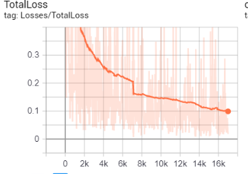
However, the results seem the same. This is because the model is not learning when there is a huge fluctuation in the loss for example

The objective is to minimize the loss function through the training. In different words, it means the model is making fewer errors. All machine learning algorithms will repeat many times the computations until the loss reach a flatter line. Minimization of this loss function depends on the learning rate ( speed the model learns). If learning rate is too high, the model does not have time to learn anything. However, on checking the learning rate defined in the model, it is 0.0002 which is low when compared to the other model. Then on further research, it is found that the model is not learning because it is trained for one class and it automatically creates another class called background. The background is trained using the regions of the training images that are not labelled as the desired classes (in your case, F1). The solution is to add training samples that include images that have both F1 and the objects that shouldn’t be recognized as F1, in the same scene. Also increasing the number of epochs should improve the precision (stackoverflow, 2019)
The project detects the single class F1 images using the Tensorflow Object Detection API. For further research the same model can be extended to overcome the challenges based on the solution given in the Challenges section. However, the model are trained with 300 images. But with more images (1000+) to train, the accuracy gets better with time.