An algorithm is a step-by-step process to achieve some outcome. When algorithms involve a large amount of input data, complex manipulation, or both, we need to construct clever algorithms that a computer can work through quickly.
A Sorting Algorithm is used to rearrange a given array or list elements according to a comparison operator on the elements. The comparison operator is used to decide the new order of element in the respective data structure.
There are many different sorting algorithms, with various pros and cons. Here are a few examples of common sorting algorithms.
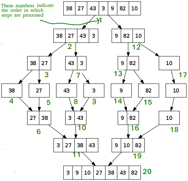
Mergesort is a comparison-based algorithm that focuses on how to merge together two pre-sorted arrays such that the resulting array is also sorted.
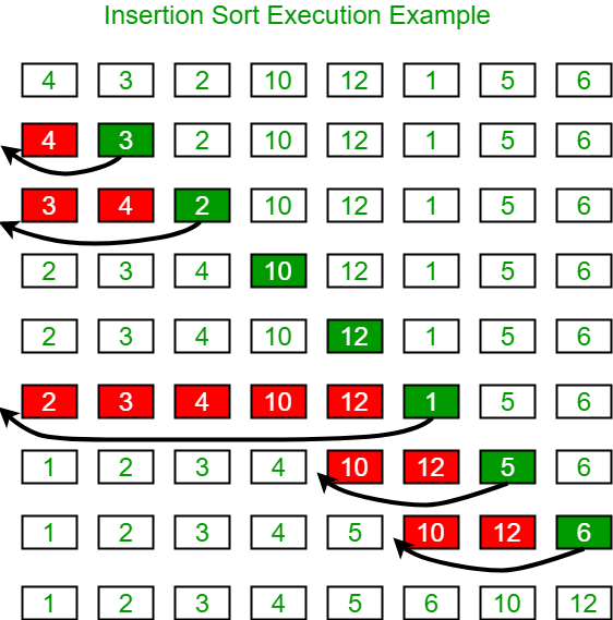
Insertion sort is a comparison-based algorithm that builds a final sorted array one element at a time. It iterates through an input array and removes one element per iteration, finds the place the element belongs in the array, and then places it there.
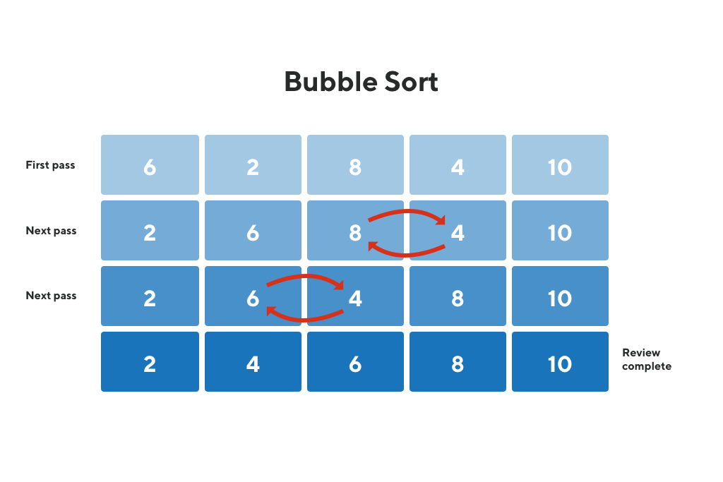
Bubble sort is a comparison-based algorithm that compares each pair of elements in an array and swaps them if they are out of order until the entire array is sorted. For each element in the list, the algorithm compares every pair of elements.
Quicksort is a comparison-based algorithm that uses divide-and-conquer to sort an array. The algorithm picks a pivot element, A[q], and then rearranges the array into two subarrays A[p…q−1], such that all elements are less than A[q], and A[q+1…r], such that all elements are greater than or equal to A[q].

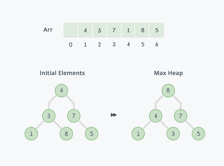
Heapsort is a comparison-based algorithm that uses a binary heap data structure to sort elements. It divides its input into a sorted and an unsorted region, and it iteratively shrinks the unsorted region by extracting the largest element and moving that to the sorted region.
Counting sort is an integer sorting algorithm that assumes that each of the n input elements in a list has a key value ranging from 0 to k, for some integer k. For each element in the list, counting sort determines the number of elements that are less than it. Counting sort can use this information to place the element directly into the correct slot of the output array.

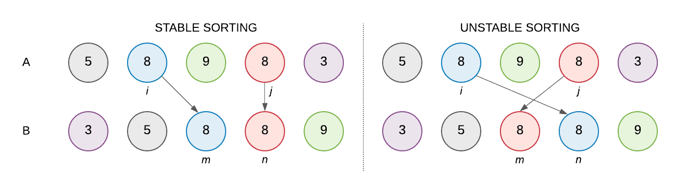
The stability of a sorting algorithm is concerned with how the algorithm treats equal (or repeated) elements. Stable sorting algorithms preserve the relative order of equal elements, while unstable sorting algorithms don’t. In other words, stable sorting maintains the position of two equals elements relative to one another.
Let’s understand the concept with the help of an example. We have an array of integers A: [ 5, 8, 9, 8, 3 ]. Let’s represent our array using color-coded balls, where any two balls with the same integer will have a different color which would help us keep track of equal elements (8 in our case):

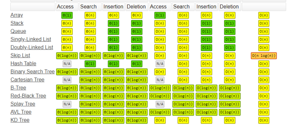
Big O notation is used in Computer Science to describe the performance or complexity of an algorithm. Big O specifically describes the worst-case scenario and can be used to describe the execution time required or the space used (e.g. in memory or on disk) by an algorithm.
O(1) describes an algorithm that will always execute in the same time (or space) regardless of the size of the input data set.
Logarithmic O(log N) — narrows down the search by repeatedly halving the dataset until you find the target value. Using binary search — which is a form of logarithmic algorithm, finds the median in the array and compares it to the target value. The algorithm will traverse either upwards or downwards depending on the target value being higher than, lower than or equal to the median.
O(N) describes an algorithm whose performance will grow linearly and in direct proportion to the size of the input data set. The example below also demonstrates how Big O favours the worst-case performance scenario; a matching string could be found during any iteration of the for loop and the function would return early, but Big O notation will always assume the upper limit where the algorithm will perform the maximum number of iterations.
O( N (log N) ) - Quasilinear time/ log-linear / Linearithmic Time. This is the time complexity of divide and conquer sorting algorithms.
In O(N log N), N is the input size (or number of elements).
log N is actually logarithm to the base 2 In divide and conquer approach, we divide the problem into sub problems(divide) and solve them separately and then combine the solutions(conquer).
O(N2) represents an algorithm whose performance is directly proportional to the square of the size of the input data set. This is common with algorithms that involve nested iterations over the data set. Deeper nested iterations will result in O(N3), O(N4) etc.
O(2^N) denotes an algorithm whose growth doubles with each addition to the input data set. The growth curve of an O(2^N) function is exponential - starting off very shallow, then rising meteorically. An example of an O(2N) function is the recursive calculation of Fibonacci numbers: