MCCL Sample Input And Output

Homogeneous tissue, R(rho), Fluence(rho,z)

Sample Input

• Please refer to the "Getting Started" pages to generate sample infiles using the command line argument "geninfiles"
• One of the infiles generated is infile_one_layer_ROfRho_FluenceOfRhoAndZ.txt
• Edit the file and specify the number of photons to be launched to be 10,000: "N": 10000,
• Run the file according to the instructions on the "Getting Started" pages for your particular system (Linux, Windows, Mac)

Sample Output

• This is the output to my Linux screen:

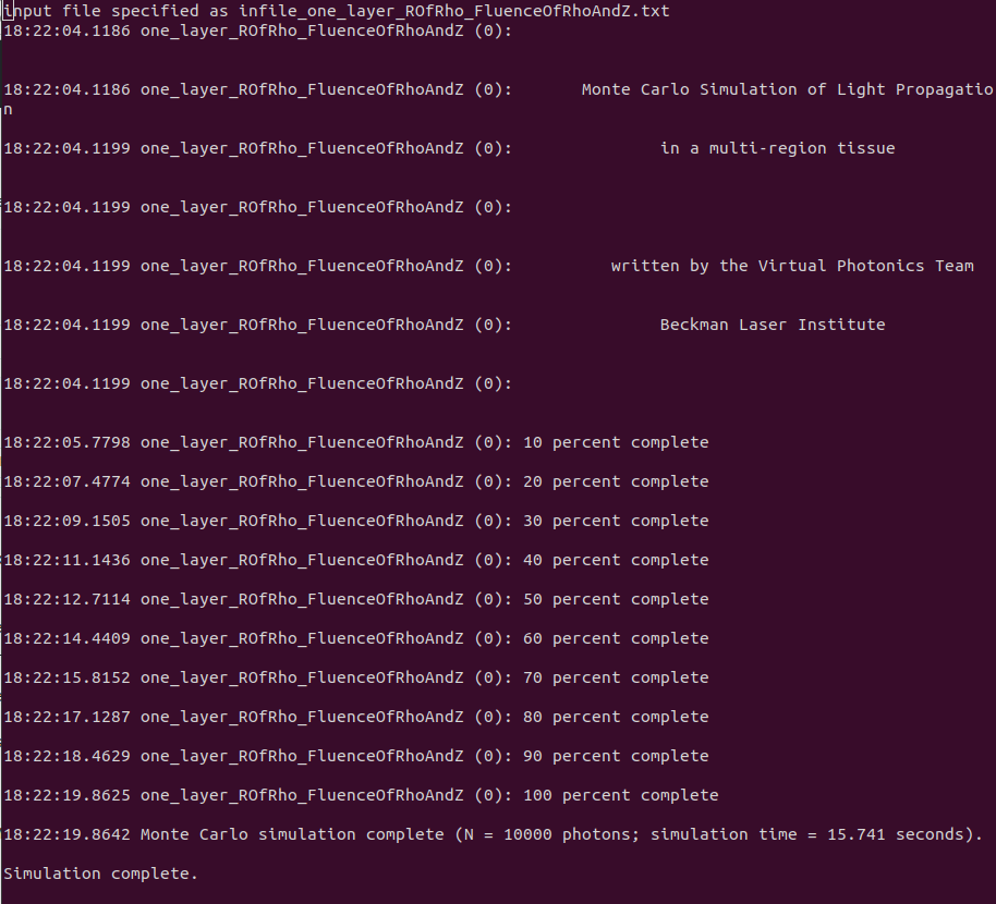
• To plot results, again follow instructions on the "Getting Started" to edit load_results_script.m and modify "datanames" to be "one_layer_ROfRho_FluenceOfRhoAndZ": datanames = { 'one_layer_ROfRho_FluenceOfRhoAndZ ' };

• Open MATLAB or Octave and run load_results_script.m. These are the plots displayed:

Comments about the plots

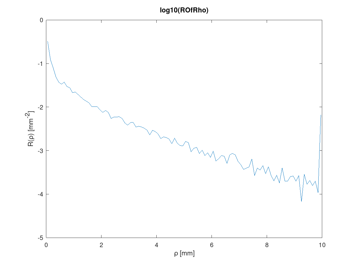
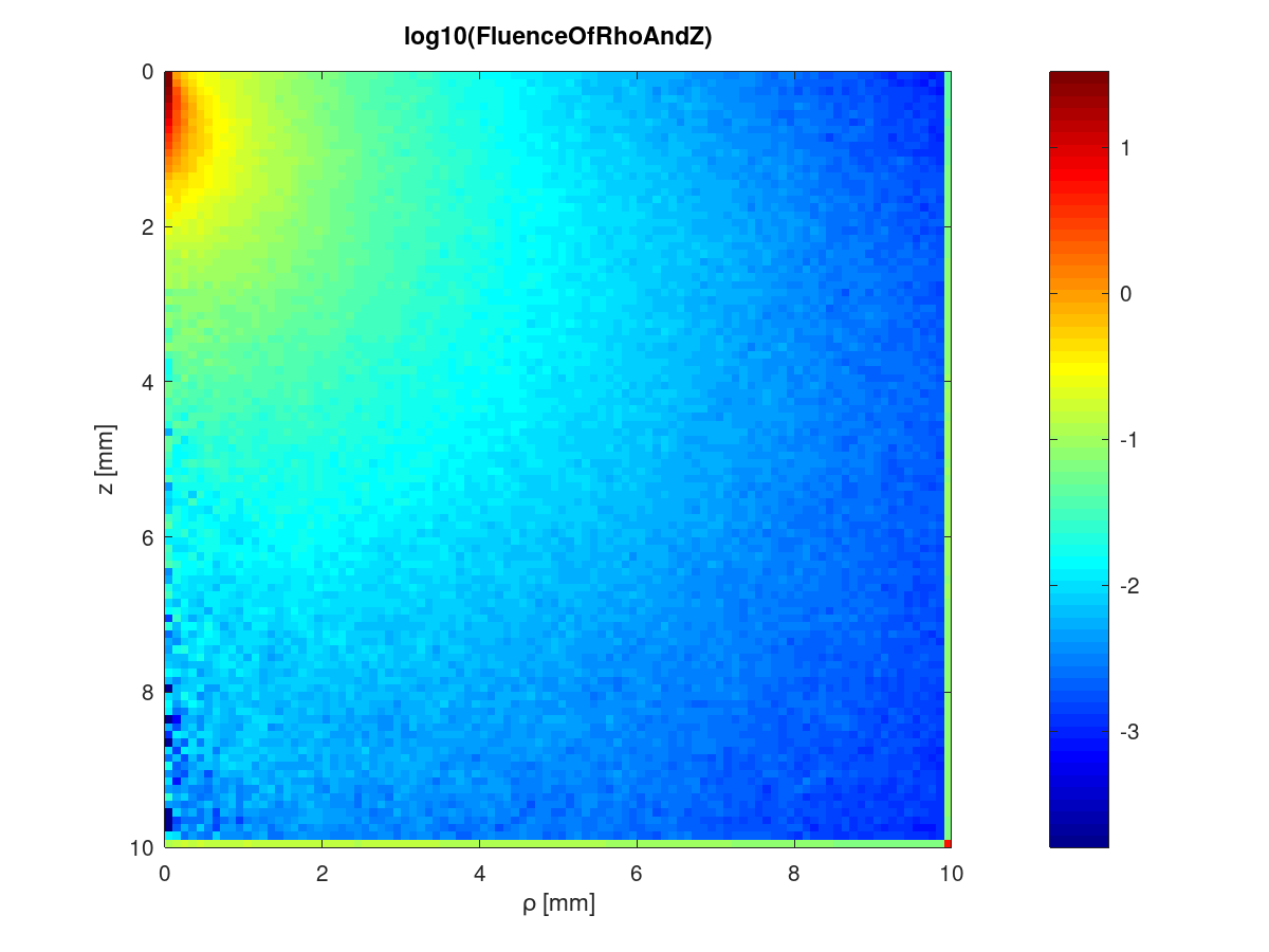
• The smoothness of both plots will increase if more photons are specified.
• Notice on the ROfRho plot that the plot rises at the last rho bin. This is because the photons that exit the tissue beyond the last rho bin will get tallied to the last rho bin. We do that so that when the tallies in all bins are un-normalized by the area of the respective circular ring and summed, total diffuse reflectance results.
• Similarly for the FluenceOfRhoAndZ, the last rho and z bins capture the tallies beyond those bins and so the edge of the fluence plot looks brighter.

Fluorescent embedded, infinite cylinder along the y-axis

Sample Input

• One of the infiles generated is infile_infinite_cylinder_AOfXAndYAndZ.txt
• Edit the file and specify the number of photons to be launched to be 10,000: "N": 10000,
• Run the file according to the instructions on the "Getting Started" pages for your particular system (Linux, Windows, Mac)
• Results of this simulation will be in the folder named "infinite_cylinder_AOfXAndYAndZ" and contain absorbed energy results as a function of Cartesian coordinates (x,y,z)
• Another infile generated using "geninfiles" is infile_fluorescence_emission_AOfXAndYAndZ_source_infinite_cylinder.txt
• Edit the file and specify the number of photons to be 10,000: "N": 10000,
• Notice that this infile has "InputFolder" defined as "infinite_cylinder_AOfXAndYAndZ" and an associated "Infile" defined as "infinite_cylinder_AOfXAndYAndZ" which identify where to find the previously generated absorbed energy results
• The "InitialTissueIndex" set to 3 specifies that the infinite cylinder region will be the fluorescent region (tissue region indices start at 0 and index through the layers, then index through the inclusions)
• The "SamplingMethod" can be set to "CDF" or "Uniform":
  • "CDF" creates a cumulative density function (CDF) from the absorbed energy map and samples the starting locations of the fluorescent photons using the CDF and starts the photons with weight=1
  • "Uniform" samples the starting locations uniformly from the fluorescent region and starts the photons with weight equal to the absorbed energy in that voxel
  • Both methods are statistically equivalent, however the advantage of one over the other is problem specific

Sample Output

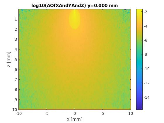
• To plot excitation results, again edit load_results_script.m and modify "datanames": datanames = { 'infinite_cylinder_AOfXAndYAndZ ' };
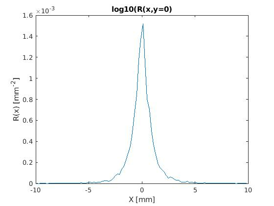
• Open MATLAB or Octave and run load_results_script.m. This is the plot displayed:

• To plot emission results, again edit load_results_script.m and modify "datanames": datanames = { 'fluorescence_emission_AOfXAndYAndZ_source_infinite_cylinder' };
• Open MATLAB or Octave and run load_results_script.m. This is the plot displayed:

Comments about the plots

• The fluorescence results have not been multiplied by quantum efficiency or any other conversion factors