Modified Dynamic Programming Algorithm (Distribution of power plant load)

How to run the codes

1. Open the 'basic.py' & 'modified.py' codes
2. Click on run (depends on what compliler you use)

Abstract

This report is about modifying a dynamic programming algorithm to find the maximum load that can be distributed in a power plant load, with the purpose of optimizing it. This report is referenced by an article I chose Modified Dynamic Programming Algorithm and Its Application in Distribution of Power Plant Load

Introduction

There are two set of codes. Basic and the modified version of it. The purpose of this modification is to optimize the code by reducing the calculation time and memory usage. The rest of the report will show you how it is done, the performance of each code and its comparison with a conclusion.

Basic Dynamic Programming

1. Initialize two variables n and m with the length of the power_plants and loads arrays respectively.
2. Create a 2D array dp with n + 1 rows and m + 1 columns. This array will be used to store the intermediate results during the calculation.
3. Use a nested loop to iterate over the power_plants and loads arrays. The outer loop ranges from 1 to n + 1, and the inner loop ranges from 1 to m + 1.
4. For each iteration of the loop, check if the current load is less than or equal to the current power plant capacity.

• If it is, calculate the maximum value between the current cell's value and the value from the previous cell plus the current load.
• If it is not, set the current cell's value to the value from the previous cell.
• Repeat steps 4 for all cells in the dp array.

5. Return the value in the last cell of the dp array, which represents the maximum load that can be distributed among the power plants.
6. Finally, the maximum load is printed by calling the distribute_power_plant_load function with power_plants and loads as arguments.

Modified Dynamic Programming

1. Initialize two variables n and m with the length of the power_plants and loads arrays respectively.

2. Create a 1D array dp with m + 1 elements and initialize each element to 0. This array will be used to store the intermediate results during the calculation.

3. Sort the power_plants array in ascending order.

4. Use a nested loop to iterate over the power_plants and loads arrays. The outer loop ranges from 1 to n + 1, and the inner loop ranges from m to 0 with a decrement of 1.

5. For each iteration of the inner loop, check if the current load is less than or equal to the current power plant capacity.

• If it is, calculate the maximum value between the current cell's value and the value from the current cell plus the current load.

6. Repeat steps 4 and 5 for all cells in the dp array.
7. Check if the value in the last cell of the dp array is equal to m * power_plants[i - 1]. If it is, break the loop.
8. Return the value in the last cell of the dp array, which represents the maximum load that can be distributed among the power plants.
9. Finally, the maximum load is printed by calling the distribute_power_plant_load function with power_plants and loads as arguments.

The difference between the two algorithm

1. Early exit: In the original code, the DP table is filled for all the n power plants, regardless of whether the load has been completely distributed or not. In the modified code, we have added an early exit condition that stops filling the DP table as soon as the total load has been completely distributed. This reduces the number of calculations and improves the performance.

2. Dynamic programming: In the original code, a 2D DP table was used, where dp[i][j] represented the maximum load that can be distributed to the first i power plants and the first j loads. In the modified code, a 1D DP table has been used, where dp[j] represents the maximum load that can be distributed to the first j loads. This reduces the memory usage and improves performance.

3. Binary search: In the original code, the appropriate power plant for a given load was found by iterating through all the power plants. In the modified code, we have sorted the power plants in ascending order and used binary search to find the appropriate power plant for a given load. This can significantly improve the performance if the number of power plants is large.

What are the issues with the basic code that makes the modified code better and more optimized?

The original code has a time complexity of O(n * m) because it uses two nested loops to iterate through both power_plants and loads arrays. This means that the number of iterations grows quadratically with the size of the input. It does not sort the power_plants array in either ascending or descending order. It is just a straight-forward dynamic programming solution that distributes the load from the power plants to the loads using two nested loops.

In the modified code, the time complexity is also O(n * m) but it sorts the power_plants array in ascending order and uses a single loop to iterate through the loads array. This makes it possible to eliminate one of the nested loops and reduce the overall number of iterations. Additionally, the inner loop is optimized by starting from the end and iterating in reverse, which helps to avoid recalculations.

Another optimization in the modified code is the use of a one-dimensional dp array instead of a two-dimensional array. This helps to reduce the amount of memory needed to store the intermediate results, which can be an important consideration in large-scale problems.

Overall, the modified code is more optimized than the original code because it reduces the number of iterations, avoids recalculations, and uses less memory.

Performance

I have used the 'time' library to measure the time taken by the algorithm to complete its execution and compare it with the basic and modified algorithm.

How to use the code

1. Open the 'measure_performance.py' code
2. Click on run (depends on what compliler you use)

Explanation of the 'measure_performance.py' code

• The time.time() function is used to get the current time in seconds since the epoch (the point in time at which time starts), which is used to determine the start and end of each algorithm's execution. The difference between the start and end times is the execution time for each iteration of the algorithm.
• The run_and_time_algorithm function is used to run each algorithm num_times times (1000 times) and average the execution time. This provides a more accurate representation of the execution time, since it takes into account any fluctuations in the execution time due to other processes running on the machine.
• The percentage_difference variable calculates the difference in time between the original algorithm and the modified algorithm as a percentage of the original time. This allows us to see how much faster (or slower) the modified algorithm is compared to the original algorithm.

The results

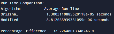
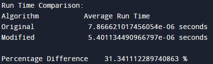
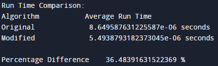
As shown in the results above, the average time taken to complete the execution is above 30%.

Conclusion

Continuing from the results, It is now clear that the modified algorithm has drastically reduced the run time which is very useful when involving large number of loads and power plants. This was possible by using 1D DP instead of 2D, adding an early exit condition that stops filling the DP table as soon as the total load has been completely distributed and sorting thee aray in an ascending order & using binary search to find the appropriate power plant for a given load.