Running InferCNV
InferCNV can be run via a simple 2-step protocol, or can be run step-by-step with customization for more exploratory purposes.
Creating an InferCNV object based on your three required inputs: the read count matrix, cell type annotations, and the gene ordering file:
# create the infercnv object
infercnv_obj = CreateInfercnvObject(raw_counts_matrix="singleCell.counts.matrix",
                                    annotations_file="cellAnnotations.txt",
                                    delim="\t",
                                    gene_order_file="gene_ordering_file.txt",
                                    ref_group_names=c("normal"))
where the ref_group_names parameter is set to the various normal-cell type (non-tumor) as defined in the cellAnnotations.txt file. See File-Definitions for more details here.
Note, if you do not have reference cells, you can set ref_group_names=NULL, in which case the average signal across all cells will be used to define the baseline. This can work well when there are sufficient differences among the cells included (ie. they do not all show a chromosomal deletion at the same place).
Note, inferCNV expects that you've already filtered out low quality cells. If you need to further impose minimum/maximum read counts per cell, you can include an additional filter, such as: min_max_counts_per_cell=c(1e5,1e6)
After creating the infercnv_obj, you can then run the standard infercnv procedure via the built-in 'infercnv::run()' method like so:
# perform infercnv operations to reveal cnv signal
infercnv_obj = infercnv::run(infercnv_obj,
                             cutoff=1,  # use 1 for smart-seq, 0.1 for 10x-genomics
                             out_dir="output_dir",  # dir is auto-created for storing outputs
                             cluster_by_groups=T,   # cluster
                             denoise=T,
                             HMM=T
                             )
The cutoff value determines which genes will be used for the infercnv analysis. Genes with a mean number of counts across cells will be excluded. For smart-seq (full-length transcript sequencing, typically using cell plate assays rather than droplets), a value of 1 works well. For 10x (and potentially other 3'-end sequencing and droplet assays, where the count matrix tends to be more sparse), a value of 0.1 is found to generally work well.
The out_dir is given an output directory name. If the directory doesn't exist, it will be created directly.
The 'cluster_by_groups' setting indicates to perform separate clustering for the tumor cells according to the patient type, as defined in the cell annotations file.
A video tutorial giving on overview of infercnv features and how to run an analysis can be found below (click on the image):
The general infercnv workflow as performed via the above infercnv::run() method operates as follows:

Setting run(denoise=TRUE) enables the de-noising procedure. Several de-noising filters are available for exploration.
Setting run(HMM=TRUE) enables the CNV predictions. There are multiple inferCNV HMM prediction methods available to explore as well.
The detailed steps of the inferCNV algorithm involve the following:
-
filtering genes: those genes found expressed in fewer than 'min_cells_per_gene' are removed from the counts matrix.
-
normalization for sequencing depth (total sum normalization): read counts per cell are scaled to sum to the median total read count across cells. Instead of a metric such as counts per million (cpm), values are counts per median sum.
-
log transformation: individual matrix values (x) are transformed to log(x+1)
-
center by normal gene expression: the mean value for each gene across normal (reference) cells is subtracted from all cells for corresponding genes. Since this subtraction is performed in log space, this is effectively resulting in log-fold-change values relative to the mean of the normal cells.
-
thresholding dynamic range for log-fold-change values. Any values with abs(log(x+1)) exceeding 'max_centered_threshold' (default=3) are capped at that value.
-
chromosome-level smoothing: for each cell, genes ordered along each chromosome have expression intensities smoothed using a weighted running average. By default, this is a window of 101 genes with a pyramidinal weighting scheme.
-
centering cells: each cell is centered with its median expression intensity at zero under the assumption that most genes are not in CNV regions.
-
adjustment relative to normal cells: The mean of the normals is once again subtracted from the tumor cells. This further compensates for differences that accrued after the smoothing process.
-
the log transformation is reverted. This makes the evidence for amplification or deletion more symmetrical around the mean. (note, with loss or gain of one copy, corresponding values 0.5 and 1.5 are not symmetrical in log space. Instead, 0.5 and 2 are symmetrical in log space. Hence, we invert the log transformation to better reflect symmetry in gains and losses).
The above generates the 'preliminary infercnv object'. The most obvious signal supporting CNVs is generally apparent in this representation. Additional filtering can be applied as a way of improving the signal to noise ratio. Also, CNV regions can be predicted using HMMs.
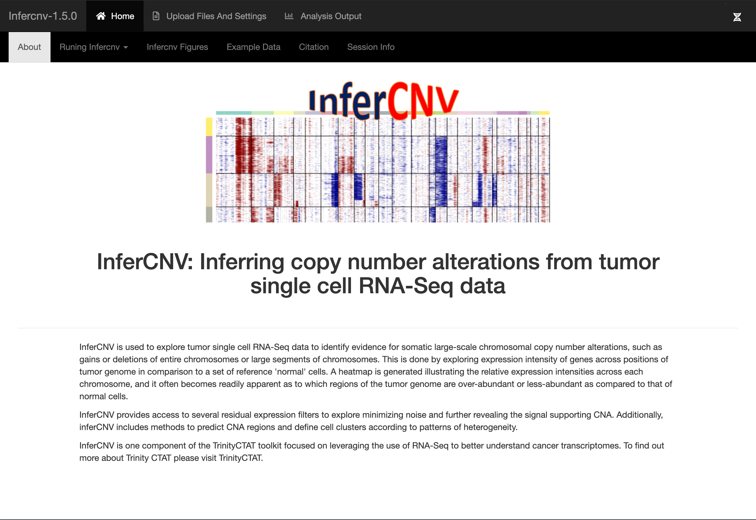
InferCNV can now be run through a WebApp that makes it easier to set the most important settings, while still allowing in detail configuration if desired. The WebApp is freely available on github.
InferCNV can also be run on the cloud using Terra. A featured workspace that illustrates running inferCNV is available here.
To interactively explore the inferCNV heatmap, see our documentation here.