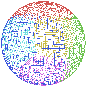
QuadSphere

QuadSphere is a small Ruby gem that implements a projection of spherical to planar coordinates, called the quadrilateralised spherical cube. It is useful for handling geographic or astronomical data, or for general mapmaking.

Background

The quadrilateralised spherical cube, or "quad sphere" for short, is a projection of the sphere onto the sides of an inscribed cube, where the distortion of the tangential (gnomonic) projection is compensated by a further curvilinear transformation. This makes it approximately equal-area, with no singularities at the poles, or anywhere; distortion is moderate over the entire sphere. This makes it well-suited for storing data collected on a spherical surface, like the Earth or the celestial sphere, as rasters of pixels: each equal-area pixel then corresponds to an equal-area region on the sphere, so numerical analysis can be performed on the pixels rather than the original surface.

This projection was proposed in 1975 in the report "Feasibility Study of a Quadrilateralized Spherical Cube Earth Data Base", by F. K. Chan and E. M. O'Neill (citation entry), and it was used to hold data for the Cosmic Background Explorer project (COBE). The quad sphere, along with a binning scheme for storing pixels along a Z-order curve, became the COBE Sky Cube format.

This is not a Sky Cube reader, though — neither the binning scheme nor the FITS format are implemented here. You should use a FITS library if you need to read COBE data. And, for current astronomical work, the quadrilateralised spherical cube projection has been superseded by HEALPix, so you should use that instead. This implementation was only created because this author had a very specific need involving storage and manipulation of spherical data — for a game, no less.

Note also that this is not the projection by Laubscher and O'Neill, 1976, which is similar to this but introduces singularities, making it non-differentiable along the diagonals.

As Chan's original report is not readily available, this implementation is based on formulae found in FITS WCS documents. Specifically: "Representations of celestial coordinates in FITS (Paper II)", Calabretta, M. R., and Greisen, E. W., Astronomy & Astrophysics, 395, 1077-1122, 2002.

Finally, bear in mind that this is not an exact projection, it's accuracy is limited — see discussion in the documentation of QuadSphere::CSC.forward_distort.

Examples

The basic usage, for converting a tuple of spherical coordinates (φ,θ) to cartesian (x,y) on a cube face, is:

require 'quad_sphere/csc'
face, x, y = QuadSphere::CSC.forward(phi, theta)

Parameters phi and theta should be given in radians. phi is the azimuthal angle, or longitude; you'll want to make it something between -π and π (or 0 and 2π, if you like). theta is the elevation angle, or (geocentric) latitude, so it should be between -π/2 and π/2. The values returned are: a face identifier (see constants in module QuadSphere), and cartesian (x,y), with each coordinate between -1 and 1.

The inverse transfomation looks, not very surprisingly, like this:

lon, lat = QuadSphere::CSC.inverse(face, x, y)

With all symbols meaning the same as before.

As a more practical example, suppose you're storing geographic data in six bitmaps of 100x100 pixels each. The following function will give you the bitmap and specific coordinates of the pixel where you should store a given latitude and longitude.

def geographic_to_storage_bin(latitude, longitude)
  # Convert both angles to radians.
  latitude = latitude*Math::PI/180
  longitude = longitude*Math::PI/180

  # Geographic latitudes are normally geodetic; we convert this to
  # geocentric because we want spherical coordinates.  The magic
  # number below is the Earth's eccentricity, squared, using the WGS84
  # ellipsoid.
  latitude = Math.atan((1 - 6.69437999014e-3) * Math.tan(latitude))

  # Apply the forward transformation...
  face, x, y = QuadSphere::CSC.forward(longitude, latitude)

  # ... then adjust x and y so they become integer coordinates on a
  # 100x100 grid, with 0,0 being top-left, as used in pictures.
  x = (100*(1+x)/2).floor
  y = 99 - (100*(1+y)/2).floor

  # And return the computed values.
  [ face, x, y ]
end

Trying the above on a few locations on Earth:

[ [ 'Accra',          5.5500,   -0.2167 ],
  [ 'Buenos Aires', -34.6036,  -58.3817 ],
  [ 'Cairo',         30.0566,  -31.2262 ],
  [ 'Honolulu',      21.3069, -157.8583 ],
  [ 'Kuala Lumpur',   3.1597,  101.7000 ],
  [ 'London',        51.5171,   -0.1062 ],
  [ 'Longyearbyen',  78.216667, 15.55   ],
  [ 'New Delhi',     28.6667,   77.2167 ],
  [ 'New York',      40.7142,  -74.0064 ],
  [ 'Quito',         -0.2186,  -78.5097 ],
  [ 'Sydney',       -33.8683,  151.2086 ],
  [ 'Ushuaia',      -54.8000,  -68.3000 ] ].each do |city, lat, lon|
  face, x, y = geographic_to_storage_bin(lat, lon)
  puts '%-12s - bitmap %d, x=%2d, y=%2d' % [city, face, x, y]
end

Gives you:

Accra        - bitmap 1, x=49, y=43
Buenos Aires - bitmap 4, x=85, y=93
Cairo        - bitmap 1, x=14, y=11
Honolulu     - bitmap 3, x=76, y=23
Kuala Lumpur - bitmap 2, x=63, y=46
London       - bitmap 0, x=49, y=93
Longyearbyen - bitmap 0, x=53, y=63
New Delhi    - bitmap 2, x=35, y=16
New York     - bitmap 4, x=67, y= 3
Quito        - bitmap 4, x=63, y=50
Sydney       - bitmap 3, x=17, y=92
Ushuaia      - bitmap 5, x=11, y=32

See more code in the examples directory, including the programs that created the graphics above. And see the API reference for the nitty gritty.