Python Cheatsheet Code Library
This is a work in progress - a collection of code/tricks useful as a reminder of the syntax.
This is generally done using pandas, which imports to a DataFrame. The following options are commonly used:
If your file has no variable names use header = None, you can manually create variable names using names=('Var1', 'Var2', 'Var3', 'Var4')
Rows can be skipped with skiprows =
More info about importing specific ranges etc available at pandas or with some code examples here
import pandas as pd
my_dataframe = pd.read_csv("C:/Users/.../csv_data.csv") # commas are default delimiter for read_csv, so you don't need to specifyAny whitespace (spaces or Tab) sep='\s+'
Tab sep='\t' or use pd.read_table where tab is the default delimiter
Multiple delimiters in regular expression [] sep='[:,|_]'
Custom delimiter sep='__'
import pandas as pd
my_dataframe = pd.read_csv("C:/Users/.../csv_data.csv", sep='__' , engine='python')import pandas as pd
my_dataframe = pd.read_excel('C:/Users/.../File.xlsx', sheetname='Sheet1')import pandas as pd
my_dataframe = pd.read_json('C:/Users/.../File.json', orient='records')To unnest / flatten JSON files in this format:
[
  {"id": -1, "label": "Not set", "description": "Blah 1"}
, {"id":  0, "label": "Not connected", "description": "Blah 2"}
, {"id":  1, "label": "Grid connect", "description": "Blah 3"}
]
You can use pandas json_normalize
my_dataframe = pd.json_normalize(json_file)for a more complicated nesting, like:
{
 "id": "ID001"
 , "comms": {
             "type": "cellular"
            , "lastHeardAt": 1630726450
            , "signalQualityDbm": -83
            , "simId": "666"
            , "apn": "optus.m2m"
            , "imsi": "666"
            , "networkId": "Optus Mobile"
            }
 , "model": "Model1"
 , "phases": {
                "count": 1
              , "grouping": [
                             {"included": ["ID001_C1"]}
                           , {"included": ["ID001_C2"]}
                           , {"included": ["ID001_C3"]}
                           , {"included": ["ID001_C4"]}
                           , {"included": ["ID001_C5"]}
                           , {"included": ["ID001_C6"]}
                            ]
              }
 , "channels": [
                {"id": "ID001_C1", "label": "Channel 1", "categoryId": 1, "categoryLabel": "Open channel", "ctRating": 60}
              , {"id": "ID001_C2", "label": "Channel 2", "categoryId": 2, "categoryLabel": "Open channel", "ctRating": 60}
              , {"id": "ID001_C3", "label": "Channel 3", "categoryId": 3, "categoryLabel": "Open channel", "ctRating": 60}
              , {"id": "ID001_C4", "label": "Channel 4", "categoryId": 2, "categoryLabel": "Clsd channel", "ctRating": 60}
              , {"id": "ID001_C5", "label": "Channel 5", "categoryId": 2, "categoryLabel": "Clsd channel", "ctRating": 60}
              , {"id": "ID001_C6", "label": "Channel 6", "categoryId": 5, "categoryLabel": "Clsd channel", "ctRating": 60}
              ]
 , "latestStatus": 1630655447
 , "firmwareVersion": "42.7.7"
 , "ReportingInterval": 30
 , "label": "Test Device 1"
 , "timezone": "Australia/Sydney"
 }
You can use the extra parameters available in json_normalize to flatten components in the way you need
my_dataframe = pd.json_normalize(json_file
                                ,record_path =['channels']   # use this to unnest lists, ie []
                                , meta=[                     # use this to keep columns
                                         'model'
                                        , "id"
                                        , "latestStatus"
                                        , "firmwareVersion"
                                        , "ReportingInterval"
                                        , "label"
                                        , "timezone"
                                        ,['comms', 'type']   # use this to extract columns within a dictionary, ie {}
                                        ,['comms' , "lastHeardAt"]
                                        ,['comms' , "signalQualityDbm"]
                                        ,['comms' , "simId"]
                                        ,['comms' , "apn"]
                                        ,['comms' , "imsi"]
                                        ,['comms' , "networkId"]
                                       ]
                                ,record_prefix='ch_'         # column name prefix for columns unnested in record_path=[]
                                ,sep='_'                     # chars to separate column name derived from concatenation of different levels of meta list
                                )
However, if you have more than one variable containing lists that you need to unlist (ie values contained in []) then you can't rely on just the record_path =['Variable name'] parameter and may have to do it another way.
If your JSON data looks like this:
{
   'duration': 2400
 , 'Metric1': [226.8, 226.8, 226.8, 226.8, 226.8, 226.8]
 , 'Metric2': [234.6, 234.7, 234.7, 234.6, 234.6, 234.7]
 , 'Metric3': [3.187, 0.0, 3.387, 0.504, 0.0, 0.897]
 , 'timestamp': 1625878800
 , 'Metric4': [0.56615, -0.00011, 0.50161, 0.08569, -5e-05, 0.07791]
 , 'Metric5': [0.56615, 0.0, 0.50161, 0.08569, 2e-05, 0.07791]
 , 'Metric6': [0.0, 0.00011, 0.0, 0.0, 7e-05, 1e-05]
}
First convert to a dataframe with json_normalise...
my_dataset = pd.json_normalize(json_file)...which will give you
	duration Metric1	                                Metric2                                    ...   timestamp  ...
0	2400	[226.8, 226.8, 226.8, 226.8, 226.8, 226.8]	[234.6, 234.7, 234.7, 234.6, 234.6, 234.7] ...   1625878800 ...
1	3600	[223.2, 223.2, 223.2, 223.2, 223.1, 223.2]	[234.7, 234.8, 234.8, 234.7, 234.7, 234.8] ...   1625882400 ...
...
To unnest all the lists
# identify non-nested variables to be 'copied down' when new rows are created by unnesting list variables
my_dataset_flat = my_dataset.set_index(['timestamp','duration'])

# unnest / transpose / reshape variables containing lists into rows
my_dataset_flat = (
                   my_dataset_flat.apply(
                                         lambda x: pd.DataFrame(x.tolist(),index=x.index)
                                                   .stack()
                                                   .rename(x.name)
                                        ).reset_index()
                  )
Which will result in
	timestamp    duration level_2	Metric1	Metric2
0	1625878800	2400	0	226.8	234.6
1	1625878800	2400	1	226.8	234.7
2	1625878800	2400	2	226.8	234.7
3	1625878800	2400	3	226.8	234.6
4	1625878800	2400	4	226.8	234.6
5	1625878800	2400	5	226.8	234.7
6	1625882400	3600	0	223.2	234.7
7	1625882400	3600	1	223.2	234.8
8	1625882400	3600	2	223.2	234.8
9	1625882400	3600	3	223.2	234.7
10	1625882400	3600	4	223.1	234.7
11	1625882400	3600	5	223.2	234.8
The code below show how to connect to SQL Server using Microsoft Active Directory credentials and return a dataframe to Python via the function sql_query_sqlserver defined below.
## Create function to query SQL Server GDW and return Dataframe

from urllib import parse
from sqlalchemy import create_engine
from sqlalchemy.sql import text
import pandas as pd

def sql_query_sqlserver(sql_query):

    # INPUT <---- SQL String
    # OUTPUT ---> Dataframe with data returned by the SQL

    # building connection string & engine
    connecting_string = 'Driver={ODBC Driver 18 for SQL Server};Server=tcp:database_path,port;Database=Database_name;Encrypt=yes;TrustServerCertificate=no;Connection Timeout=30;Authentication=ActiveDirectoryIntegrated'
    params = parse.quote_plus(connecting_string)
    engine = create_engine("mssql+pyodbc:///?odbc_connect=%s" % params)

    # connect to SQL server
    with engine.connect() as conn:
        result = conn.execute(text(sql_query))
        rows = result.fetchall()

    # pushing results to a Dataframe
    df = pd.DataFrame(rows, columns=result.keys())
    return df
Now call the function sending passthrough SQL to SQL Server and returning dataframe my_df
# Pull data from table in SQL Server
sql_string = """
  select *
  FROM schema.table
  WHERE
"""

my_df = sql_query_sqlserver(sql_string)Creates dataframe my_df from SQLite database MnB_sandpit table titanic_train
import sqlite3
import pandas as pd

conn = sqlite3.connect(r"C:/Users/GordonWallace/sqlite/MnB_sandpit.sqlite3")

my_df = pd.read_sql('select * from titanic_train', conn)Use index = False to prevent export of row index (which exports as a column)
Use header = False to prevent export of column index (which exports as the first row)
import pandas as pd
my_dataframe.to_csv('C:/Users/.../data_export.csv', index = False, header=False )Delimiter can be defined using sep = '', in this case pipe
import pandas as pd
my_dataframe.to_csv('C:/Users/.../data_txt_export.txt', sep ='|', index = False )Use index = False to prevent export of row index (which exports as a column)
Some other funky things like freeze_panes=(1,1) or restrict variables exported with columns=["Var1", "Var2"]
import pandas as pd
my_dataframe.to_excel('C:/Users/.../data_excel_export.xlsx', sheet_name="My Sheet", index = False, columns=["Var1", "Var2"] )Print first 5 rows of data as text in console. Use .head(-5) to see first and last 5 rows
my_dataframe.head(5) Lists all Variables, their type, non-null count & index position
my_dataframe.info()Summary Statistics of Numeric Variables. Adding include='all' gives summaries for character variables too.
my_dataframe.describe(include='all')Lists all variables in the dataframe with a count of all the nulls
my_dataframe.isnull().sum()These two are equivalent, with rows selection criteria first, then columns to display - all returned if nothing specified
my_dataframe[(my_dataframe['var1'] > 0.5) & (my_dataframe['var2'] == 1)][["var3","var1","var2"]]
my_dataframe.loc[(my_dataframe['var1'] > 0.5) & (my_dataframe['var2'] == 1),["var3","var1","var2"]]
These approaches can also include other functions like str.contains here selecting rows where var4 contains the phrase 'shadow' (case insensitive)
my_dataframe[my_dataframe.var4.str.contains('shadow', case=False)]** Note: take care when changing a dataframe that is a copy of another dataframe, as the 'copy' is normally just an alias pointing to the same underlying object. This means changing the copy can also change the original. ie if df2 = df1 then renaming a column in df2 can also rename the same column in df1 unless you are careful to create a new underlying object.
Use inplace=True to overwrite existing variable names for df1 and df2 rather than create a new dataframe with the new names
my_dataframe.rename(columns={'Var1' : 'New_Var1', 'Var2' : 'New_Var2', 'Var3' : 'New_Var3'}, inplace=True) # this will change all dataframes pointing to the same underlying object
my_dataframe = my_dataframe.rename(columns={'Var1' : 'New_Var1', 'Var2' : 'New_Var2', 'Var3' : 'New_Var3'}) # this will only change my_dataframe (inplace=False is default)

my_dataframe.columns = ['New_Var1', 'New_Var2', 'New_Var3'] # must include all variables for this methodmy_dataframe["Var1"] = my_dataframe["Var1"].astype(str) # single variable
my_dataframe = my_dataframe.astype({'Var1': str, 'Var2': int}) # multiple variablesThe following tries to automatically convert to more dataframe appropriate types (objects to str etc.) and make more null friendly
my_dataframe = my_dataframe.convert_dtypes()
my_dataframe = my_dataframe.infer_objects() The following code drops the variables Var1 and Var2
my_dataframe = my_dataframe.drop(columns=['Var1', 'Var2']) # changes made to my_dataframe only
my_dataframe.drop(columns=['Var1', 'Var2'], inplace=True) # changes made to all dataframes pointing to underlying object, ie if my_dataframe is a copy of another df This is the equivalent of case when in SQL, except you need to do it in 2 steps.
# define the function
def my_function(x):
  if x['type1'] == 'fire' and x['against_dark'] == x['against_dragon']: return 10
  elif x['type1'] != 'normal' and (x['type2'] == 'poison' or x['type2'] == 'flying'): return 5
  else: return 0

# call the function on your dataframe
my_dataframe['points'] = my_dataframe.apply(my_function, axis=1)
You can also do with a lambda function (a one-shot function that doesn't get named and kept for use later)
This code replaces nulls with the value 'missing' so it is treated like a category so doesn't break various calcs / can be converted to a dummy variable with get_dummies
my_dataframe = my_dataframe.fillna('missing')A lot of machine learning algorithms in python can't handle categorical variables, so these have to be converted to dummy variables with 1s or 0s flagging each level of the variable. Painful, but luckily there is a quick way of doing it!
my_dataframe = pd.get_dummies(my_dataframe)Create Rank variable Var3_rank based on Var3 across whole dataframe
my_dataframe['Var3_rank'] = my_dataframe['Var3'].rank(method='dense')Create Rank variable Var3_rank based on Var3 within each category of Var1 and Var2
my_dataframe['Var3_rank'] = my_dataframe.groupby(['Var1','Var2'])['Var3'].rank(method='dense')Sort dataframe by Var1, Var2, Var3
my_dataframe = my_dataframe.sort_values(by = ['Var1','Var2','Var3'], ascending = [True, True, True], na_position = 'first')Create counter variable counter_var within each category of Var1 by ascending Var2 and descending Var3
You can also do this in SQL using the sqldf library
row_number() over (partition by Var1 order by Var2 asc, Var3 desc) as counter_varHere the \ is just used to split over rows to make the code more readable
my_dataframe['counter_var'] = my_dataframe.sort_values(['Var2','Var3'], ascending=[True,False]) \
             .groupby(['Var1']) \
             .cumcount() + 1
Other examples of how to do this in various situations here
There is a good summary of the usual suspects here including the methods below.
ie for fox = "tHe qUICk bROWn fOx."
fox.lower() converts to all lower case
fox.upper() converts to all upper case
line = ' this is the content '
line.strip() removes all leading and trailing spaces. There is also rstrip() and lstrip
line.replace('t','') will remove all the 't' characters
You can also fill / pad a string using
'435'.rjust(10, '0') to get 0000000435
There are a few ways of doing this - don't forget that python indexing starts at 0 and that the first number is inclusive while the second is exclusive (annoying, I know). So myString[2 : 7] includes everything from index 2 (character 3) to index 6 (character 7)
myString = "Mississippi"
print(myString[4 :  ]) # issippi
print(myString[  : 8]) # Mississi
print(myString[2 : 7]) # ssiss
or using slicer
print(myString[slice(4, 99)]) # issippi
print(myString[slice(0, 8)])  # Mississi
print(myString[slice(2, 7)])  # ssiss
This example uses regular expressions to extract the title from a name field in the format Wallace, Mr. Gordon
For more info on regex look here or here
all_data['Title'] = all_data.Name.str.extract(r',\s*([^.]*)\s*\.', expand=False)The awesome pandasql package is basically the same as sqldf in R. It creates a temporary SQLite database in memory and lets you use SQL commands to manipulate your dataframes, including all the SQL favourites - joins, subqueries, case when, aggregation functions (sum, avg, count etc), window functions (rank over partition by etc)
from pandasql import sqldf

df = sqldf(
"""
SELECT
   Var1
  ,Var2
  ,count(*) as num_rows
  ,avg(Var3) as Var3_avg
FROM my_dataframe
WHERE Var1 = 'xyz'
group by 1,2
having Var3_avg > 100
;
"""
)
Create counter variable counter_var within each category of Var1 by ascending Var2 and descending Var3
from pandasql import sqldf

df = sqldf(
"""
SELECT
   Var1
  ,Var2
  ,Var3
  ,row_number() over (partition by Var1 order by Var2, Var3 desc) as counter_var
FROM my_dataframe
;
"""
)One of the fastest and most convenient ways of exploring and manipulating complex data in Python is to turn dataframes into database tables in SQLite. You can then use the pretty amazing free database IDE DBeaver to get a first look at your data, with all the ease of SQL and an interface designed for quick analysis. You can then embed any SQL used to manipulate data into Python via passthrough queries (just like the old days in SAS!) and of course bring back into a dataframe if needed.
First, create the SQLite database (most systems already have SQLite installed for other purposes)
## Create local SQLite database for storing and viewing dataframes
import sqlite3

conn = sqlite3.connect(r"C:/Users/GordonWallace/sqlite/MnB_sandpit.sqlite3")
conn.close()
Next, send dataframes to SQLite to become database tables (here done via function df_to_sqlite):
## Send Dataframe to SQLite database table

import sqlite3
import os
import pandas as pd

def df_to_sqlite(database_name, database_directory, table_name, dataframe):

    # INPUT <---- Database name & location, new table name, dataframe
    # OUTPUT ---> nil

    database_path = os.path.join(database_directory, f"{database_name}.sqlite3")
    conn = sqlite3.connect(database_path)

    # Create SQL from dataframe
    dataframe.to_sql(table_name, conn, if_exists='replace', index=False)

    # Commit the changes and close the database connection
    conn.commit()
    conn.close()
then call the function to send dataframe my_df to table titanic_train in SQLite database MnB sandpit:
df_to_sqlite("MnB_sandpit", "C:/Users/GordonWallace/sqlite", "titanic_train", my_df)Once the tables exist, you can use passthrough SQL to manipulate them (including all the normal SQL tricks such as creating, altering, updating tables, grouping by, window functions etc):
# Send pass-through SQL to SQLite
con = sqlite3.connect("C:/Users/GordonWallace/sqlite/MnB_sandpit.sqlite3")
cursor = con.cursor()

cursor.execute(
"""
alter table titanic_train
add high_risk_flag
"""
)
con.commit()

cursor.execute(
"""
update titanic_train
set high_risk_flag = case when Sex = 'male' and Pclass = 3 then 'High Risk' else null end
;
"""
)
con.commit()

cursor.close()
To bring back from an SQLite table into a dataframe is pretty simple. The code below creates dataframe my_df from SQLite database MnB_sandpit table titanic_train
import sqlite3
import pandas as pd

conn = sqlite3.connect(r"C:/Users/GordonWallace/sqlite/MnB_sandpit.sqlite3")

my_df = pd.read_sql('select * from titanic_train', conn)The grand daddy of charts in python is matplotlib but this is often unwieldy, so luckily there are more user friendly packages like seaborn and dexplot, the latter being my fave as it is easy and beautiful (www.dexplo.org/dexplot/). You can create some pretty great interactive visualizations with altair (https://altair-viz.github.io/index.html) but the syntax is not that intuitive - for special occasions.
This produces a simple X vs Y text table of means in the Console
import pandas as pd
pd.crosstab(my_dataframe.Sex, my_dataframe.Pclass, values=my_dataframe.Survived, aggfunc='mean')

Pclass         1         2         3
Sex
female  0.968085  0.921053  0.500000
male 0.368852 0.157407 0.135447You can use a list to create X vs Y vs Z text table of means in the Console
import pandas as pd
pd.crosstab([train_raw.Sex, train_raw.Embarked], train_raw.Pclass, values=train_raw.Survived, aggfunc='mean')

Pclass                  1         2         3
Sex    Embarked
female C         0.976744  1.000000  0.652174
       Q         1.000000  1.000000  0.727273
       S         0.958333  0.910448  0.375000
male   C         0.404762  0.200000  0.232558
       Q         0.000000  0.000000  0.076923
S 0.354430 0.154639 0.128302Easily create summary stats for combos of categorical variables
train_raw.groupby(["Sex","Pclass"])['Survived'].describe().reset_index() Sex Pclass count mean std min 25% 50% 75% max
0 female 1 94.0 0.968085 0.176716 0.0 1.0 1.0 1.0 1.0
1 female 2 76.0 0.921053 0.271448 0.0 1.0 1.0 1.0 1.0
2 female 3 144.0 0.500000 0.501745 0.0 0.0 0.5 1.0 1.0
3 male 1 122.0 0.368852 0.484484 0.0 0.0 0.0 1.0 1.0
4 male 2 108.0 0.157407 0.365882 0.0 0.0 0.0 0.0 1.0
5 male 3 347.0 0.135447 0.342694 0.0 0.0 0.0 0.0 1.0
To create a simple 100% stacked
import dexplot as dxp
dxp.count(
           data=train_raw
          ,val='Sex'   # X-axis
          ,split='Survived'
          ,normalize='Sex'  # 100% stacked by including both col & val variables
          ,stacked=True
          ,title='Survival proportion by Sex'
          )
This can very easily be changed to be across multiple variables
dxp.count(
           data=train_raw
          ,val='Pclass'   # X-axis
          ,split='Survived'
          ,col='Sex'
          ,normalize=['Pclass','Sex']  # 100% stacked by including both col & val variables
          ,stacked=True
          ,title='Survival proportion by Sex & Pclass'
          )
...or even in a grid
dxp.count(
           data=train_raw
          ,val='Pclass'   # X-axis
          ,split='Survived'
          ,row='Embarked'
          ,col='Sex'
          ,normalize=['Pclass','Sex','Embarked']  # 100% stacked by including both col & val variables
          ,stacked=True
          ,title='Survival proportion by Sex, Pclass & Embarked'
          )
Again dexplot makes things super easy here.
import dexplot as dxp
dxp.hist(val='Age', data=train_raw, row='Sex', split='Survived', bins=15)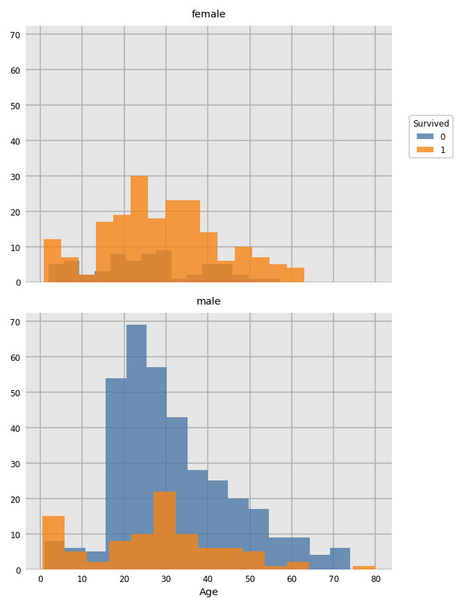
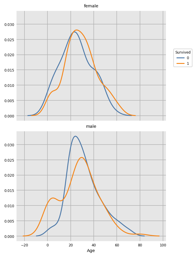
For a smoothed KDE plot use the following (oops about negative age...)
dxp.kde(
          x='Age'
        , data=train_raw[train_raw.Age.notnull()]  # remove nulls as kde doesn't like missing values
        , row='Sex'
        , split='Survived'
        )
import dexplot as dxp
dxp.scatter(x='Age', y='Fare', data=train_raw, split='Survived', row='Sex')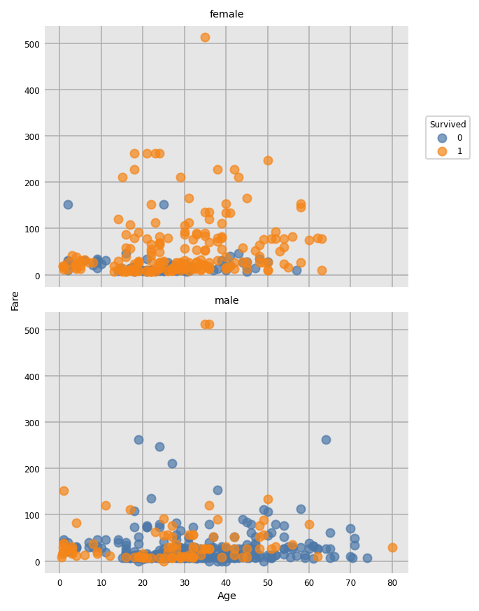
A very useful way of quickly visualising your data with a grid of scatter plots with histograms on the diagonal.
import seaborn as sns
sns.set(rc={"figure.dpi":150, 'savefig.dpi':150}) # set the resolution here
sns.pairplot(all_data, hue='Survived', palette='coolwarm')
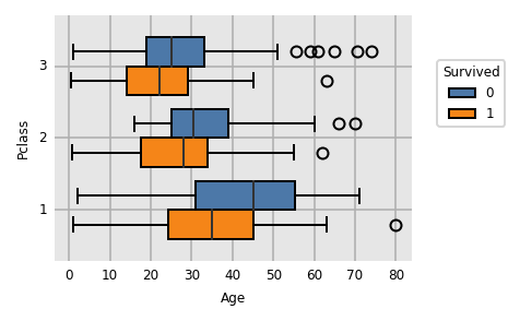
Boxplot
dxp.box(
         x='Age', y='Pclass', split='Survived'
        ,data=train_raw[train_raw.Age.notnull()]  # remove nulls as kde doesn't like missing values
        )
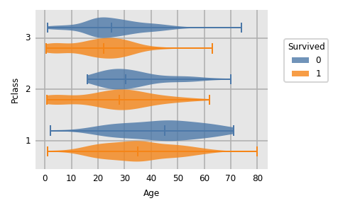
Violin plot
dxp.violin(
            x='Age', y='Pclass', split='Survived'
           ,data=train_raw[train_raw.Age.notnull()]  # remove nulls as kde doesn't like missing values
           )
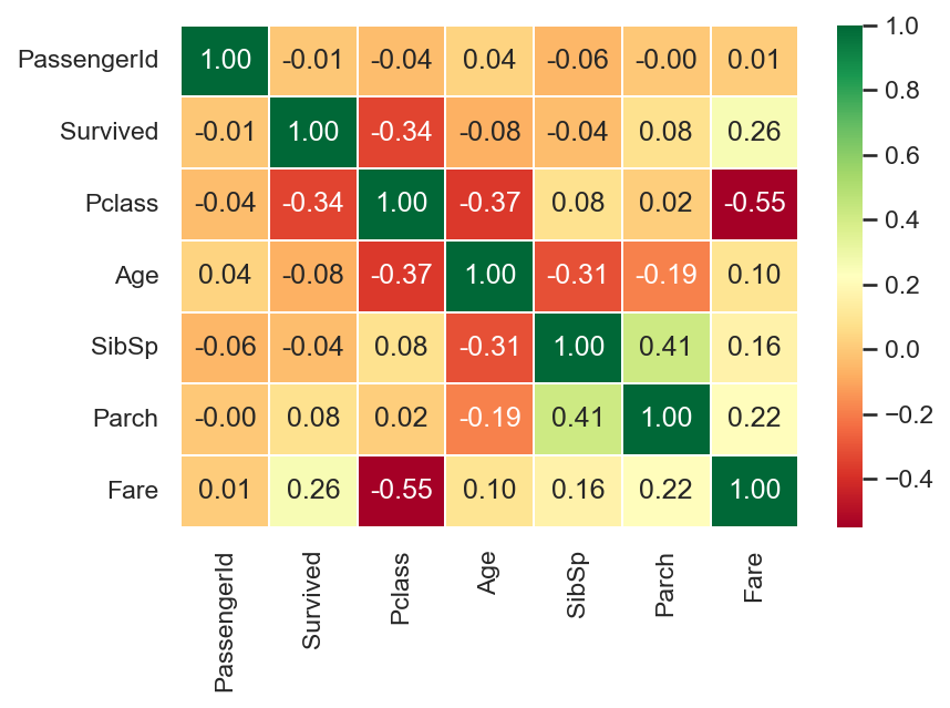
seaborn also has some great chart options, including this useful correlation heatmap for continuous variables
import seaborn as sns
sns.set(rc={"figure.dpi":150, 'savefig.dpi':150}) # use to set resolution of chart created
sns.heatmap(
            data=train_raw.corr()
           ,annot=True
           ,cmap='RdYlGn'  # colour scheme
           ,linewidths=0.2
           ,fmt='.2f'  # set decimal points
           )
There are a few different datascience-y packages, but the classic is scikit-learn, or sklearn which can do a lot of things, but can be a bit idiosyncratic. For example dependent and independent variables generally need to be in different dataframes.
You can use train_test_split to split the modeling data into 4 dataframes - training & validation data, each of which is also split into datasets for dependent y and independent x variables
from sklearn.model_selection import train_test_split
x_train, x_test, y_train, y_test = train_test_split(
                                                      train.loc[:, train.columns != 'Survived']  # list the features / independent variables
                                                     ,train["Survived"]    # list the target / dependent variable
                                                     ,test_size=0.3        # this sets aside 30% of the rows for the validation dataframe
                                                     ,stratify=train["Survived"]  # this ensures sample proportions of dependent var values are the same as the population
                                                     ,random_state=123456  # a seed so results can be replicated
                                                     )
If you really need to preserve sample size and are going to trust cross-validation to prevent overfitting and do without a test dataset, then you can easily manually split the x and y data
x_train     = train.loc[:, train.columns != 'Survived']
y_train_pre = train.loc[:, train.columns == 'Survived']
y_train = y_train_pre.squeeze() # convert one column dataframe to series for modellingBelow is code for a Random Forest approach to a classic classification problem, the Kaggle Titanic survival competition. A Random Forest is a collection of Decision Trees each run on a subset of rows and variables which are then combined to make the final prediction. They work best when the component trees are independent (hence subsampling of both rows & columns), so beware correlated or closely related variables.
This code:
- Assumes you've already split the data into train and test samples (see above)
- Uses a grid of model parameters to run multiple models using different combos of these to 'hypertune' the parameters (this doesn't necessarily protect you from overfitting, so use realistic param ranges and keep an eye on those fit stats!)
- Provides model fit statistics and plots (precision, recall, accuracy, confusion matrix, ROC curve, variable importance, tree plot)
- Uses the final model to classify dataset not used in the training & testing
####### Random Forest Classifier
from sklearn.ensemble import RandomForestClassifier # Random Forest Classifier
from sklearn.model_selection import GridSearchCV    # Use grid of parameters to tune hyperparameters
from sklearn.metrics import classification_report

# Create the parameter grid - each combo of these values will be used to fit a separate model, so don't go too crazy!
param_grid = {
     'bootstrap': [True]
    ,'max_depth': [3, 4, 5]         # max number of levels in trees
    ,'max_features': [7,12,15]      # max number of features to use to generate each tree
    ,'min_samples_leaf': [5,10,15]  # min number of cases required to justify a leaf's existence
    ,'min_samples_split': [10, 20]  # min number of cases required to justify a node split's existence
    ,'n_estimators': [100, 200]     # number of trees in the forest
    }
The code below will probably give you a TLDR moment, but shows model fit deets for all the combos of params in the grid.
# Precision = What proportion of positive identifications was actually correct? = TP / (TP + FP)
# Recall    = What proportion of actual positives was identified correctly?     = TP / (TP + FN)
scores = ['precision','recall']

for score in scores:
    print("# Tuning hyper-parameters for %s" % score)
    print()

    # Instantiate the grid search model
    grid_search = GridSearchCV(
                                 estimator = RandomForestClassifier()
                                 , param_grid = param_grid
                                 , cv = 5
                                 , n_jobs = -1
                                 , verbose = 2
                                 , scoring='%s_macro' % score
                                 )

    # Fit the grid search to the data
    grid_search.fit(x_train, y_train)

    print("Best parameters set found on development set:")
    print()
    print(grid_search.best_params_)
    print()
    print("Grid scores on development set:")
    print()
    means = grid_search.cv_results_['mean_test_score']
    stds = grid_search.cv_results_['std_test_score']
    for mean, std, params in zip(means, stds, grid_search.cv_results_['params']):
        print("%0.3f (+/-%0.03f) for %r"
              % (mean, std * 2, params))
        print()

    print("Detailed classification report:")
    print()
    print("The model is trained on the full development set.")
    print("The scores are computed on the full evaluation set.")
    print()
    y_true, y_pred = y_test, grid_search.predict(x_test)
    print(classification_report(y_true, y_pred))
    print()
The bit at the bottom is probably of most interest:
...
Detailed classification report:

The model is trained on the full development set.
The scores are computed on the full evaluation set.

              precision    recall  f1-score   support

         0.0       0.78      0.80      0.79       128
         1.0       0.70      0.67      0.68        87

    accuracy                           0.75       215
   macro avg       0.74      0.74      0.74       215
weighted avg       0.75      0.75      0.75       215


RandomForestClassifier(max_depth=4, max_features=4, min_samples_leaf=20, min_samples_split=60)
{'bootstrap': True, 'max_depth': 4, 'max_features': 4, 'min_samples_leaf': 20, 'min_samples_split': 60, 'n_estimators': 100}
If that is too much info, you can just get the results for the 'best' combo of parameters
# Diagnostics of grid search
print(grid_search.best_estimator_)
print(grid_search.best_params_)
I like to then re-run to model in a more conventional sense using these 'best' parameters so you have access to the normal model fit stats.
# Re-run model with best parameters just to get access to more model diagnostics
model = grid_search.best_estimator_

# Use model to predict test set
y_test_pred = model.predict(x_test)
y_train_pred = model.predict(x_train)


### Model fit stats
from sklearn.metrics import classification_report, accuracy_score, plot_confusion_matrix, confusion_matrix, plot_roc_curve

# ROC for Training and Test on one chart (store the first graph as 'roc' & use its axis to plot second graph)
roc = plot_roc_curve(model, x_train, y_train, name = 'Train')
roc = plot_roc_curve(model, x_test,  y_test,  name = 'Test', ax = roc.ax_)
plt.show()
To get an idea of the importance of the variables to the model:
## Variable importance
feature_names = x_train.columns

importances = list(model.feature_importances_)
std = np.std([tree.feature_importances_ for tree in model.estimators_], axis=0)
forest_importances = pd.Series(importances, index=feature_names)

fig, ax = plt.subplots()
forest_importances.plot.bar(yerr=std, ax=ax)
ax.set_title("Feature importances using MDI")
ax.set_ylabel("Mean decrease in impurity")
fig.tight_layout()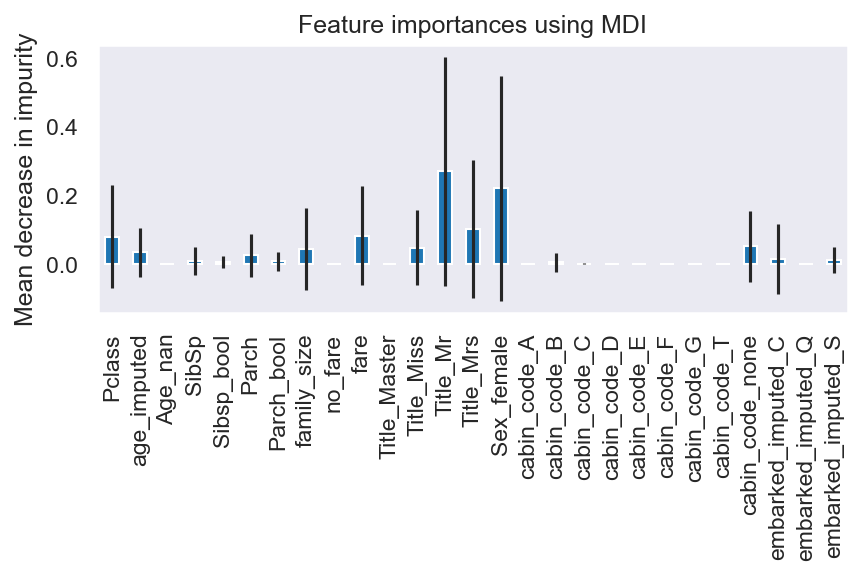
To get an idea of accuracy (precision, recall etc.):
# Classification Report
class1 = classification_report(y_test, y_test_pred)
print("Classification Report:",)
print (class1)

accuracy = accuracy_score(y_test, y_test_pred)
# print(f'Out-of-bag score estimate: {model.oob_score_:.2}')
print(f'Mean accuracy score: {accuracy:.2}')
Classification Report:
precision recall f1-score support
0.0 0.78 0.80 0.79 128
1.0 0.70 0.67 0.68 87
accuracy 0.75 215
macro avg 0.74 0.74 0.74 215
weighted avg 0.75 0.75 0.75 215
Mean accuracy score: 0.75
Although the Random Forest is a combo of (probably) hundreds of trees, it can be useful to plot individual trees for reality checking
## Draw tree diagram for one tree from the Random Forest
import graphviz
from sklearn.tree import export_graphviz
from sklearn import tree

dot_data= export_graphviz(model.estimators_[0]  # choose which tree to chart here (this is the first one)
                          ,out_file = None
                          ,feature_names = x_train.columns
                          ,class_names = ['Died','Survived']
                          ,filled = True
                          ,rounded = True
                          ,special_characters = True, impurity = True)
graph = graphviz.Source(dot_data, format='png')
graph 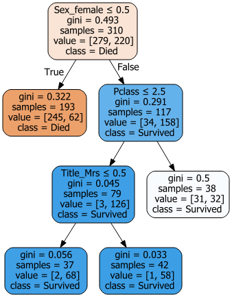
For the ever useful Confusion Matrix (2 ways to create this):
# Confusion Matrix using Seaborn
# cm = pd.DataFrame(confusion_matrix(y_train, y_train_pred))
cm = pd.DataFrame(confusion_matrix(y_test, y_test_pred))
cm_plt = sns.heatmap(cm, annot=True,linewidths=0.2, fmt='.0f')
cm_plt.set( xlabel = "Predicted", ylabel = "Actual")

# Confusion matrix straight from sklearn
plot_confusion_matrix(model, x_test, y_test)
plt.show()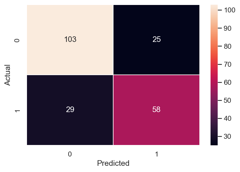
Use model to predict as yet unseen data and export to CSV
# Use model to predict to_predict dataset
y_to_predict_pred = model.predict(x_to_predict.loc[:,x_to_predict.columns != 'PassengerId']) # exclude PassengerId as wasn't used in model
y_to_predict_pred = y_to_predict_pred.astype('int') # for some reason prediction is float... convert to int

output = pd.DataFrame({'PassengerId': x_to_predict.PassengerId, 'Survived': y_to_predict_pred})
output.to_csv('D:/Maven & Boyg/Blah/rf_predictions.csv', index=False)
print("Your submission was successfully saved!")