Time Freq
HRV analysis by means of frequency-domain methods can only yield information about how IBI signal power is distributed in the frequency domain. They provide no insight into the temporal evolution of the spectrum. Methods used to allow simultaneous viewing of both time and frequency information are often termed time-frequency analysis. Like frequency-domain analysis, time-frequency HRV analysis quantifies VLF, LF, and HF related measures. The two primary types of time-frequency analysis used are the windowed Fourier transform (also called short-time Fourier transform, STFT) and the continuous wavelet transform [36]. To include spectral estimation methods other than the Fourier transform, the term windowed periodogram will be used in place of windowed Fourier transform. This generalization allows the inclusion of the windowed Burg periodogram and windowed Lomb-Scargle periodogram.
The windowed power spectrum is an extension of the basic PSD. As the term implies, the data is broken down into consecutive (overlapping or not) segments or windows. The PSD is then computed for each segment. This is similar to the technique use by Bartlett and Welch. However, those methods lose any temporal information by averaging all PSD’s into a single PSD. Unlike Welch’s method, the windowed periodogram can use other techniques to compute the PSD, e.g. Burg periodogram. Plotting PSD values onto a two-dimensional plane with frequency and time as the vertical and horizontal axes respectively produces a spectrogram (Figure 2.5).
Two alternatives are the windowed Burg periodogram and the windowed Lomb-Scargle periodogram [37, 38]. For the windowed Burg periodogram the entire data series is first resampled and then broken into segments of equal lengths. Finally, the PSD is computed for each segment using the Burg periodogram. The windowed Lomb-Scargle periodogram is computed in almost the same manner. First, the data is broken into segments of equal lengths of time [26]. Due to the uneven sampling of IBI’s, each segment can contain differing number of data points. Finally, the LSP for each segment is computed.
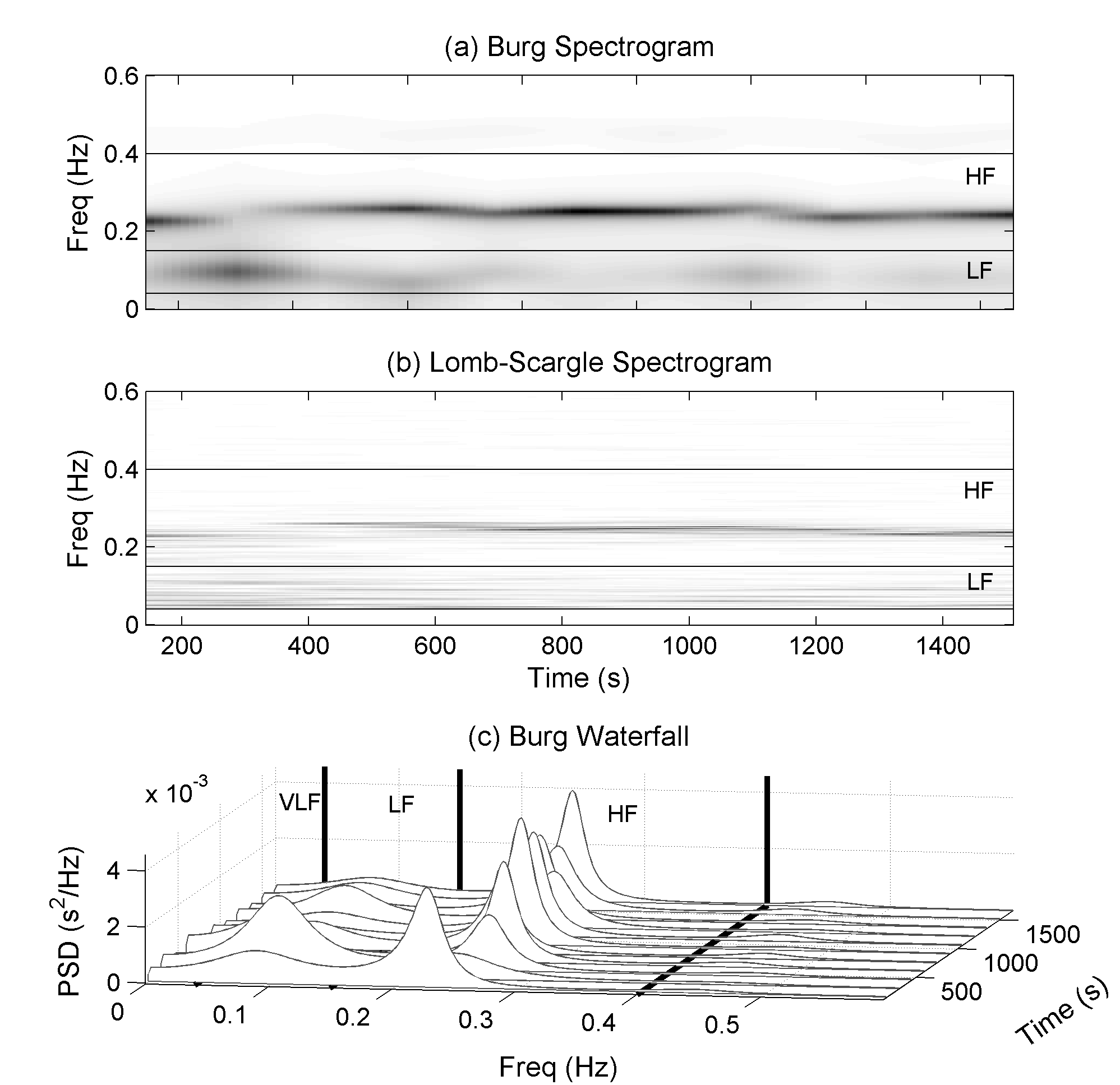
Figure 2.5 – Spectrogram and waterfall plot for windowed periodograms. Plots generated using preprocessed IBI from healthy human. Plots include (a) Spectrogram using windowed Bug periodogram. (b) Spectrogram using windowed LSP (c) Waterfall plot containing Burg periodograms of each five minute segment of IBI.
HRV quantification from time-frequency analysis using windowed periodograms can be accomplished two ways. The first method computes an averaged or global power spectrum and then calculates typical frequency-domain HRV measures ,e.g., LF, HF, LFHF. Averaging the power spectrum eliminates any time resolution and defeats some of the purpose of time-frequency analysis, but it provides a way to help control variances by averaging many power spectrums [39]. Alternatively, HRV measures can be calculated for each segment, and then an average HRV measure computed. The second method produces discretely instantaneous frequency-domain measures that are a function of time, e.g., LF(t) and LFHF(t).
From the LFHF instantaneous time series, another index can be extracted called the ratio of LFHF ratios (rLFHF) [37]. This measure represents the “global” sympathetic-parasympathetic equilibrium [37]. Imagine a line drawn through LFHF =1 on the instantaneous LFHF plot. Above this line (LFHF >1) there is a sympathetic dominance. Below this line (LFHF <1) there is a parasympathetic dominance. The rLFHF ratio is obtained by calculating the ratio of the bounded area above the line LFHF=1 to the bounded area below.
Wavelet transforms are a relatively recent, but enormously popular tool for analyzing and compressing many types of time signals. The term wavelet implies a small wave and is of finite length and energy [40]. Like Fourier transform the wavelet transform separates a signal into its fundamental components. However, unlike the Fourier transform, wavelet transforms can be applied to non-stationary signals and are not limited to a single set of basis waveforms for signal decomposition. Fourier transforms rely on the sinusoid waveform, whereas wavelet transforms have an infinite set of basis waveforms or mother wavelets as long as they satisfy predefined mathematical criteria. This property may provide access to information that could be obscured by methods like Fourier analysis [41]. Acharya, et al. state that “bio-signals usually exhibit self-similarity patterns in their distribution, and a wavelet which is akin to its fractal shape would yield the best results in terms of clarity and distinction of patterns. [41]”
The following summary of Acharya’s [2] understanding of wavelet transform concepts provides an efficient explanation. The wavelet transform correlates a mother wavelet with sections of the original signal to produce wavelet coefficients. The mother wavelet is shifted/translated in time to generate a set of coefficients along the time signal. Next the mother wavelet is contracted or dilated to create coefficients along the time series at varying time scales. Here the term scale is analogous to frequency or more precisely the pseudo frequency (average frequency). Scaled wavelets are normalized so each one contains the same amount of energy. The scale can be thought of as the wavelet width and the translation as its location in time. Larger scale values represent smaller wavelet size and thus higher frequencies.
This research is concerned with the continuous wavelet transform (CWT), the discrete wavelet transform (DWT), and discrete wavelet packet transform (DWPT). The major differences between the three are how the wavelet function is scaled and translated.
For a given signal x(t) and wavelet function , the CWT coefficients are given by
Equation (2.16)
where is the complex conjugate of the mother wavelet , α is the dilation parameter, and τ is the location parameter. The bivariant function W(τ,α) shows the similarity of x(t) to a wavelet scaled by α at a given time τ [20]. Theoretically the CWT wavelet coefficients are calculated for infinitesimally small translations and scale factors. However, practical implementations of the CWT must balance the number of translations and scales to produce acceptable computational times. Most programmatic implementations of the CWT allow the user to specify the number of scales to use for computation. Plotting CWT coefficients onto a two-dimensional plane with scale and location as the vertical and horizontal axes produces a scalogram.
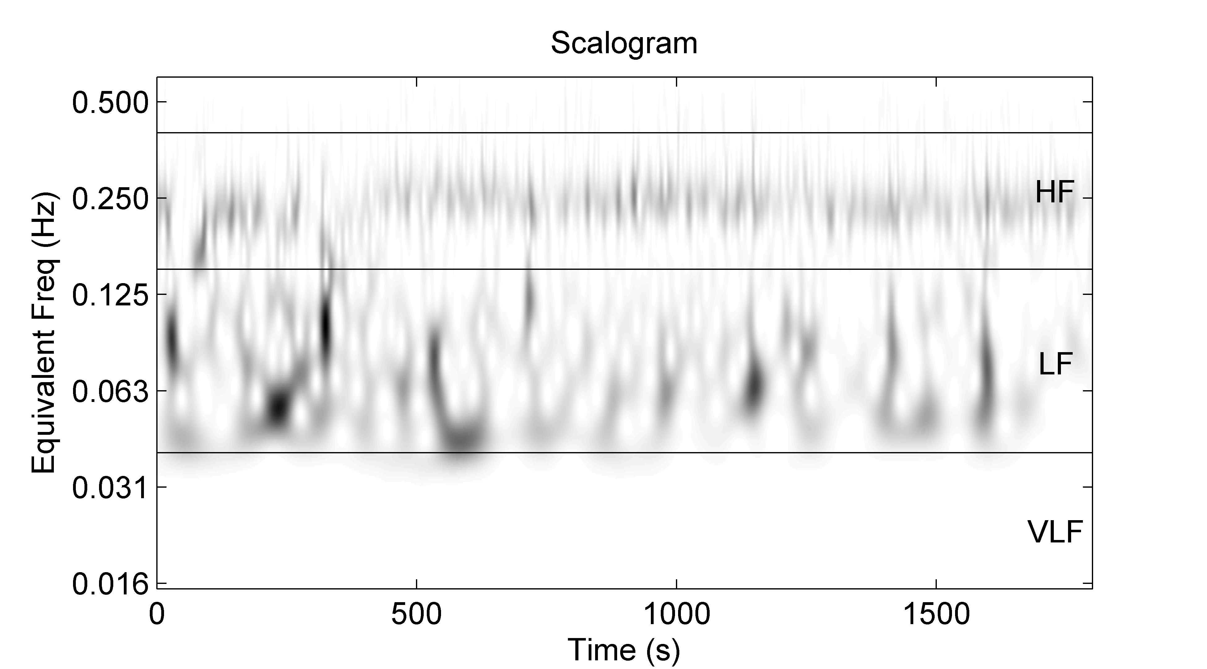
Figure 2.6 – CWT scalogram of IBI data. CWT computed using preprocessed IBI from healthy human with DOG2 wavelet [42]. The frequency axis is displayed using a log scale and represents the equivalent frequency of CWT scales [42].
In the case of DWT and DWPT, the scaling and translations are done in a less smooth or more discrete manner. Scaling and translating for the DWT are based on powers of 2 or dyadic blocks, e.g., 21, 22, etc. The dilation function is often represented as a tree of low and high pass filters. The first step of the tree decomposes the original signal into detail (high frequency) and approximation (low frequency) components. Detail and approximation components for three levels of decomposition are represented in Figure 2.7-a by A and D. Only the approximations are further split into finer components in the DWT. For DWPT both branches of the tree are split into finer components. Figure 2.7-b shows the tree for DWPT for 3 levels of decomposition.

Figure 2.7 – DWT decomposition tree. Decomposition trees showing the breakdown of an arbitrary original signal into three levels using (a) discrete wavelet transform and (b) wavelet packet transform. Horizontal axis shows frequency range as a fraction of the Nyquist frequency. DWPT can extract all frequency bands with equal resolution. Diagram modified from Tanaka and Hargens [43].
Quantification of HRV measures from time-frequency analysis by CWT is accomplished in a similar manner to that employed for the windowed periodogram. Similar in that both can use either the instantaneous or global power spectrums [44]. To obtain HRV measures using instantaneous power methods, the squared modulus of the wavelet coefficients is integrated over the desired frequency band [f1 f2]. To integrate over a frequency band wavelet scales must be changed to frequencies. The time-scale map (scalogram) must be interpreted in terms of a time-frequency map (spectrogram). The instantaneous power of the frequency band [f1 f2] is given by
Equation (2.17)
The wavelet equivalent to an averaged periodogram is the global wavelet spectrum and is given by
Equation (2.18)
- finish equations
- finish inline eq
- add cross refs to other pages