From the japanese word Maki-e, which is a technique to sprinkle lacquer with gold and silver powder. Data is the gold and silver of our age, so let's spread it out beautifully on the screen!
Check out the documentation here!
If you use Makie for a scientific publication, please cite our JOSS paper the following way:
Danisch & Krumbiegel, (2021). Makie.jl: Flexible high-performance data visualization for Julia. Journal of Open Source Software, 6(65), 3349, https://doi.org/10.21105/joss.03349
BibTeX entry:
@article{DanischKrumbiegel2021,
  doi = {10.21105/joss.03349},
  url = {https://doi.org/10.21105/joss.03349},
  year = {2021},
  publisher = {The Open Journal},
  volume = {6},
  number = {65},
  pages = {3349},
  author = {Simon Danisch and Julius Krumbiegel},
  title = {Makie.jl: Flexible high-performance data visualization for Julia},
  journal = {Journal of Open Source Software}
}Please consider using the backends directly. As explained in the documentation, they re-export all of Makie's functionality. So, instead of installing Makie, just install e.g. GLMakie directly:
julia>]
pkg> add GLMakie
You may check the installed version with:
]st GLMakieStart using the package:
using GLMakieMakie and its backends all live in the Makie monorepo. This makes it easier to change code across all packages. Therefore, dev'ing Makie almost works as with other Julia packages, just, that one needs to also dev the sub packages:
]dev --local Makie # local will clone the repository at ./dev/Makie
]dev dev/Makie/MakieCore dev/Makie/GLMakie dev/Makie/CairoMakie dev/Makie/WGLMakie dev/Makie/RPRMakie
To run the tests, you also should add:
]dev dev/Makie/ReferenceTestsFor more info about ReferenceTests, check out its README
The following examples are supposed to be self-explanatory. For further information check out the documentation!
x = 1:10
fig = lines(x, x.^2; label = "Parabola")
axislegend()
save("./assets/parabola.png", fig, resolution = (600, 400))
figSimilar to the one on this link
x = -2pi:0.1:2pi
approx = fill(0.0, length(x))
set_theme!(palette = (; patchcolor = cgrad(:Egypt, alpha=0.65)))
fig, axis, lineplot = lines(x, sin.(x); label = L"sin(x)", linewidth = 3, color = :black,
    axis = (; title = "Polynomial approximation of sin(x)",
        xgridstyle = :dash, ygridstyle = :dash,
        xticksize = 10, yticksize = 10, xtickalign = 1, ytickalign = 1,
        xticks = (-π:π/2:π, ["π", "-π/2", "0", "π/2", "π"])
    ))
translate!(lineplot, 0, 0, 2) # move line to foreground
band!(x, sin.(x), approx .+= x; label = L"n = 0")
band!(x, sin.(x), approx .+= -x .^ 3 / 6; label = L"n = 1")
band!(x, sin.(x), approx .+= x .^ 5 / 120; label = L"n = 2")
band!(x, sin.(x), approx .+= -x .^ 7 / 5040; label = L"n = 3")
limits!(-3.8, 3.8, -1.5, 1.5)
axislegend(; position = :ct, bgcolor = (:white, 0.75), framecolor = :orange)
save("./assets/approxsin.png", fig, resolution = (600, 400))
figx = y = -5:0.5:5
z = x .^ 2 .+ y' .^ 2
set_theme!(colormap = :Hiroshige)
fig = Figure()
ax3d = Axis3(fig[1, 1]; aspect = (1, 1, 1),
perspectiveness = 0.5, azimuth = 2.19, elevation = 0.57)
ax2d = Axis(fig[1, 2]; aspect = 1)
pltobj = surface!(ax3d, x, y, z; transparency = true)
heatmap!(ax2d, x, y, z; colormap = (:Hiroshige, 0.5))
contour!(ax2d, x, y, z; linewidth = 2, levels = 12, color = :black)
contour3d!(ax3d, x, y, z; linewidth = 4, levels = 12,
transparency = true)
Colorbar(fig[1, 3], pltobj)
colsize!(fig.layout, 1, Aspect(1, 1.0))
colsize!(fig.layout, 2, Aspect(1, 1.0))
resize_to_layout!(fig)
save("./assets/simpleLayout.png", fig)
figset_theme!().
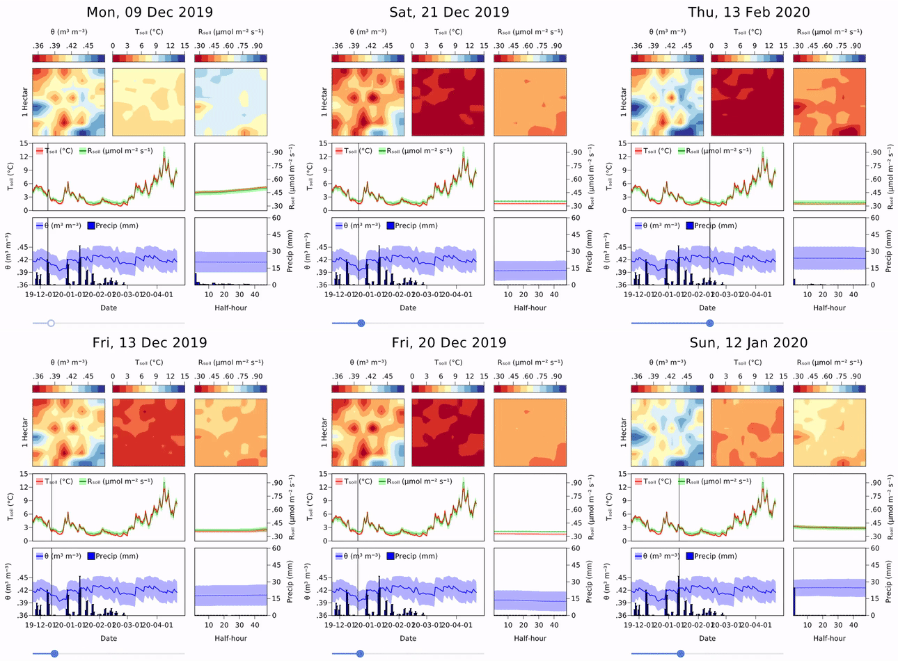
Interactive example by AlexisRenchon:
Example from InteractiveChaos.jl
You can follow Makie on twitter to get the latest, outstanding examples:


