A collection of MATLAB scripts.
The input values for each function are generally not validated other than their lengths. If an error such as division by 0 occurs, it will propagate. Please refer to each function's help documentation for additional information.
- Tridiagonal LU Decomposition Matrix Solver
a. Example - Least-Square Plot Using QR Decomposition
a. Example - Natural Clamped Cubic Spline
a. Example - Inverse Quadratic Interpolation
a. Example
This script solves Ax = d for x using LU decomposition for the square tridiagonal matrix A.
A square tridiagonal matrix A has the following structure:
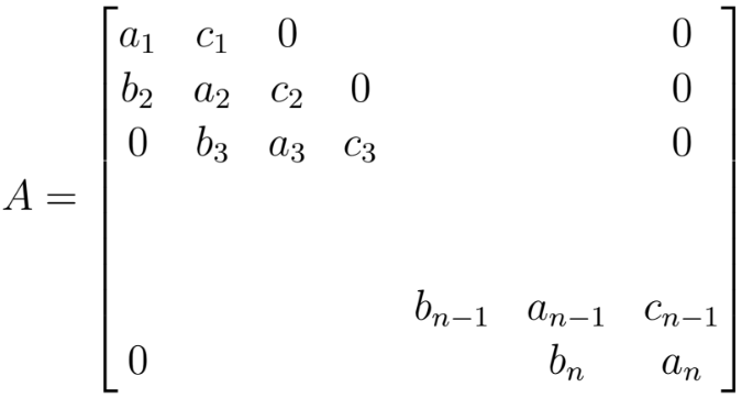
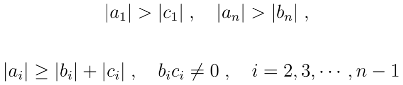
The a, b and c variables are used as vector inputs for the script. The values must meet the following criteria for the script to work:
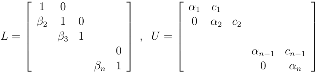
The output includes vector x and vector z such that z = Ux. It also includes vectors alpha and beta such that:
>> [alpha, beta, z, x] = tridiag_lu_decomp([2;2;2;2;2], [1;1;1;1;1], [1;1;1;1;1], [3;4;4;4;3])

alpha =
    2.0000    1.5000    1.3333    1.2500    1.2000

beta =
         0    0.5000    0.6667    0.7500    0.8000

z =
    3.0000    2.5000    2.3333    2.2500    1.2000

x =
     1     1     1     1     1
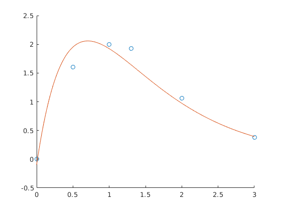
This script solves Ax = y for the n x 1 vector x in the least-square sense using QR decomposition. It also plots the least-square fit function along with the input coordinates for comparison.
The input n x 1 basis functions (with m x 1 input t) are used to form the m x n matrix A. For example, for n = 2 basis functions b_1(t) = e^-t and b_2(t) = e^-2t with m = 3 input coordinates given by t = [0; 1; 2] and y = [0; 2; 1.06], we get the following 3 x 2 matrix:
    [ e^0   e^0  ]
A = [ e^-1  e^-2 ]
    [ e^-2  e^-4 ]
>> [x] = lsquare_plot_with_qr([0;.5;1;1.3;2;3], [0;1.6;2;1.93;1.06;0.38], {@(t)exp(-t), @(t)exp(-2*t)})

x =
    8.3282
   -8.4245
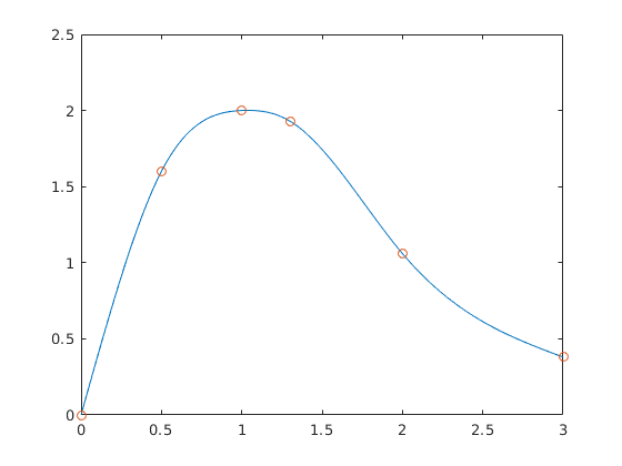
This script interpolates given coordinates to find a natural clamped cubic spline function and plots the results.
The output includes vectors for the intially unknown variables in the spline function S. See the help docs for more info.
>> [m,a,b] = nat_clamped_cubic_spline([0;.5;1;1.3;2;3], [0;1.6;2;1.93;1.06;0.38])

m =
         0   -6.9356   -1.0575   -3.4675    1.7072         0

a =
         0    3.7780    6.7195    3.1617    0.7755

b =
    3.7780    4.0881    6.6067    1.3151    0.3800
This script interpolates a given function at the given points using the inverse quadratic method until the user says to stop. If the numbers appear to diverge or have converged, the interpolating should be stopped.
>> x = inverse_quad_interp([0.6, 0.7, 0.9], @(x)x^5 - cos(x)^2)
    0.8568    0.6000    0.7000

To stop interpolating, type 0, else 1: 1
    0.8494    0.8568    0.6000

To stop interpolating, type 0, else 1: 1
    0.8477    0.8494    0.8568

To stop interpolating, type 0, else 1: 1
    0.8477    0.8477    0.8494

To stop interpolating, type 0, else 1: 1
    0.8477    0.8477    0.8477

To stop interpolating, type 0, else 1: 1
    0.8477    0.8477    0.8477

To stop interpolating, type 0, else 1: 0

x =
    0.8477    0.8477    0.8477