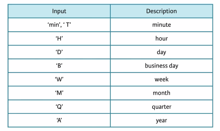
3. Time series in pandas

1 Indexing pandas time series

1.1 Using pandas to read date time objects

1.2 Product sales CSV

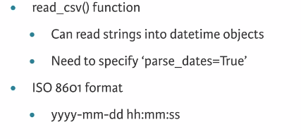
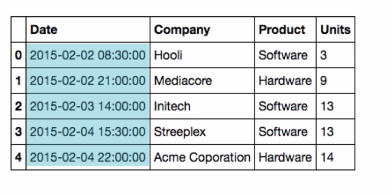
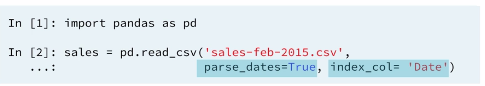
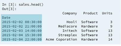
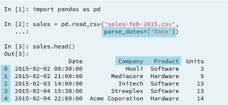
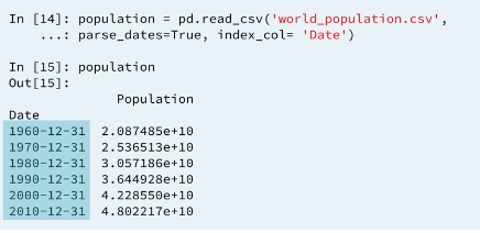
Since we know that the csv file contains at least one column of Datetimes we can tell read_csv to parse all compatible columns as Datetime objects with parse_dates = True option. Further, we are going to use the Date column as the index.

1.3 Parse dates

1.4 Selecting single datetime

1.5 Selecting whole day

1.6 partial datetime string selection

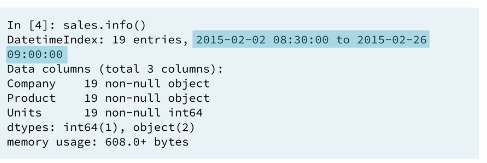
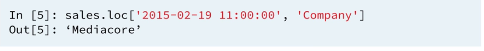
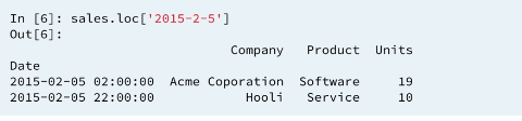
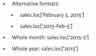
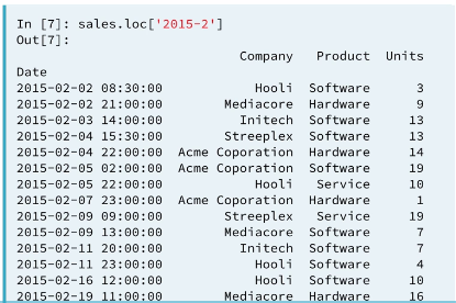
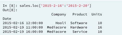
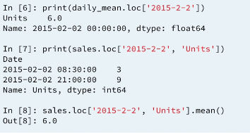
Pandas time series support "partial string" indexing. What this means is that even when passed only a portion of the datetime, such as the date but not the time, pandas is remarkably good at doing what one would expect. Pandas datetime indexing also supports a wide variety of commonly used datetime string formats, even when mixed.

1.7 Selecting Whole month

1.8 Slicing using dates/times

1.9 Converting strings to datetime

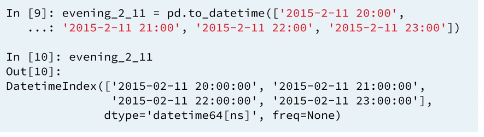
The pandas to_datetime function can convert strings in ISO 8601 format into pandas datetime object.

Nice example from the later chapter

EXERCISE Cleaning and tidying datetime data

1.10 Reindexing DataFrame

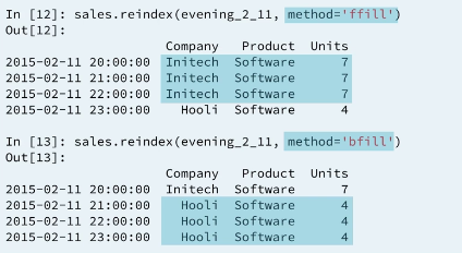
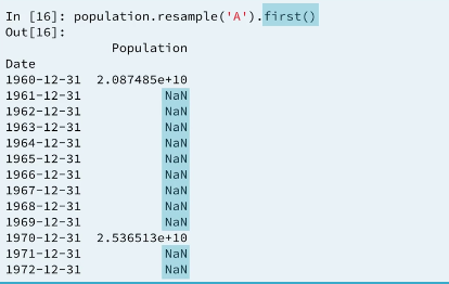
We sometimes need to re index the series or dataframe. Re-indexing involves providing a new index and matching data as required

1.11 Filling missing values

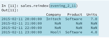
When using reindex with missing entries we can override the default behavior for felling with NAN using the argument method='ffill' which means forward fill. The empty entries are filled using the nearest proceeding non null entire in each column. We can also specify method='bfill' for backward fill. The opposite of Forward fill Which is better depends on the context of your data processing task. So pandas gives as some flexibility.

Example 1 : Creating and using a DatetimeIndex

The pandas Index is a powerful way to handle time series data, so it is valuable to know how to build one yourself. Pandas provides the pd.to_datetime() function for just this task. For example, if passed the list of strings ['2015-01-01 091234','2015-01-01 091234'] and a format specification variable, such as format='%Y-%m-%d %H%M%S, pandas will parse the string into the proper datetime elements and build the datetime objects.

In this exercise, a list of temperature data and a list of date strings has been pre-loaded for you as temperature_list and date_list respectively. Your job is to use the .to_datetime() method to build a DatetimeIndex out of the list of date strings, and to then use it along with the list of temperature data to build a pandas Series.

Instructions

• Prepare a format string, time_format, using '%Y-%m-%d %H:%M' as the desired format.
• Convert date_list into a datetime object by using the pd.to_datetime() function. Specify the format string you defined above and assign the result to my_datetimes.
• Construct a pandas Series called time_series using pd.Series() with temperature_list and my_datetimes. Set the index of the Series to be my_datetimes.

# Prepare a format string: time_format
time_format = '%Y-%m-%d %H:%M'

# Convert date_list into a datetime object: my_datetimes
my_datetimes = pd.to_datetime(date_list, format=time_format)  

# Construct a pandas Series using temperature_list and my_datetimes: time_series
time_series = pd.Series(temperature_list, index=my_datetimes)

Example: 2 Reindexing the Index

Reindexing is useful in preparation for adding or otherwise combining two time series data sets. To reindex the data, we provide a new index and ask pandas to try and match the old data to the new index. If data is unavailable for one of the new index dates or times, you must tell pandas how to fill it in. Otherwise, pandas will fill with NaN by default.

In this exercise, two time series data sets containing daily data have been pre-loaded for you, each indexed by dates. The first, ts1, includes weekends, but the second, ts2, does not. The goal is to combine the two data sets in a sensible way. Your job is to reindex the second data set so that it has weekends as well, and then add it to the first. When you are done, it would be informative to inspect your results.

INSTRUCTIONS:

• Create a new time series ts3 by reindexing ts2 with the index of ts1. To do this, call .reindex() on ts2 and pass in the index of ts1 (ts1.index).
• Create another new time series, ts4, by calling the same .reindex() as above, but also specifiying a fill method, using the keyword argument method="ffill" to forward-fill values.
• Add ts1 + ts2. Assign the result to sum12.
• Add ts1 + ts3. Assign the result to sum13.
• Add ts1 + ts4, Assign the result to sum14.

# Reindex without fill method: ts3
ts3 = ts2.reindex(ts1.index)

# Reindex with fill method, using forward fill: ts4
ts4 = ts2.reindex(ts1.index, method='ffill')

# Combine ts1 + ts2: sum12
sum12 = ts1 + ts2

# Combine ts1 + ts3: sum13
sum13 = ts1 + ts3

# Combine ts1 + ts4: sum14
sum14 = ts1 + ts4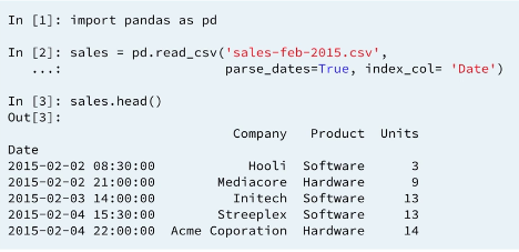

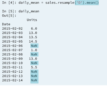
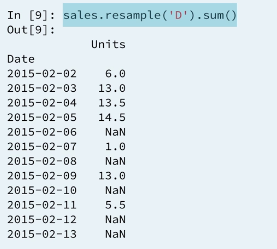
2 Resampling pandas time series

2.1 Sales data

2.2 Resampling

2.3 Aggregating means

There are three important things to notice here.

• First, The method resample needs a string to specify frequency. here D stands for daily.
• Second, The resample method is chained with the mean method. It is best practice to follow resample with some statistical method in this way.
• Third, The result is a dataframe with daily frequency for February, 2015 with the average number of units sold each day. The columns company and product are non-numerical and hence are ignored. Missing days are filled with NaN but that can be changed.

2.4 Verifying

2.5 Method chaining

Remember, when using resample, we use method chaining. In this case, we chain resample with the sum method to get daily totals

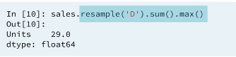
We can build long chains of methods if we want.

2.6 Resampaling strings

The result has three columns because the count method applies for string also. The week ending February 8th had the most individual sales.

2.7 Resamplaing frequencies

2.8 Multiplying frequencies

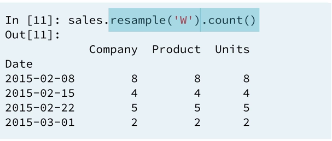
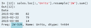
Notice, the first entry is February 8, this is the same value as the first row when using w.By default the '2w' offset is aligned by Sundays and February 8th was the second Sunday of the month in 2015.

2.9 Upsampling

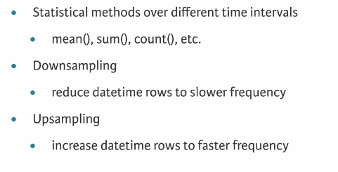
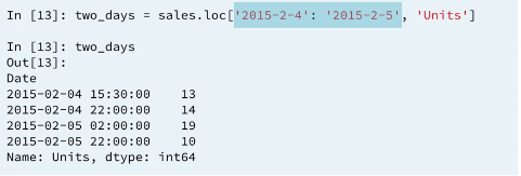
Up to now we have been downsampling. Downsamplig uses a corsal time index with fewer samples. For instance, down sampling a statistic from daily to weekly data. The opposite is upsampling. Making a finer time index with more samples. For instance, upsampling from daily to hourly data.

As an example, Lets fill in the blanks for unit sold every four hours on February 4th and February 5th.

2.10 Upsampling and filling

Example 3: Resampling and frequency

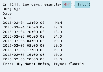
Pandas provides methods for resampling time series data. When downsampling or upsampling, the syntax is similar, but the methods called are different. Both use the concept of 'method chaining' - df.method1().method2().method3() - to direct the output from one method call to the input of the next, and so on, as a sequence of operations, one feeding into the next.

For example, if you have hourly data, and just need daily data, pandas will not guess how to throw out the 23 of 24 points. You must specify this in the method. One approach, for instance, could be to take the mean, as in df.resample('D').mean().

In this exercise, a data set containing hourly temperature data has been pre-loaded for you. Your job is to resample the data using a variety of aggregation methods to answer a few questions.

INSTRUCTIONS:

• Downsample the 'Temperature' column of df to 6 hour data using .resample('6h') and .mean(). Assign the result to df1.
• Downsample the 'Temperature' column of df to daily data using .resample('D') and then count the number of data points in each day with .count(). Assign the result df2.

# Downsample to 6 hour data and aggregate by mean: df1
df1 = df['Temperature'].resample('6h').mean()

# Downsample to daily data and count the number of data points: df2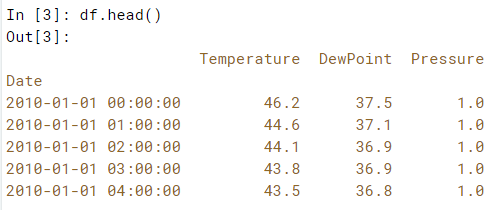
df2 = df['Temperature'].resample('D').count()

Example 4 : Separating and resampling

LINK

3 Manipulating pandas time series

3.1 Sales data

For now we are not going to use the date column as the index and instead use the default integer range as an index.

3.2 String method

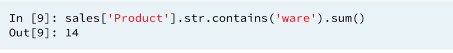
We can work with the string column as a whole using the .str attribute.

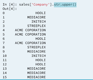
Notice that the column is not transformed in place but a new series with only upper case letters is returned.

3.2.1 Substring matching

3.2.2 Boolean arithmetic

3.2.3 Boolean reduction

3.3 Datetime methods

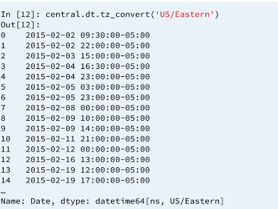
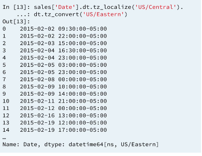
Similar to the .str attribute the .dt attribute is used for specialized datetime transformations.

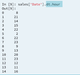
.dt.hour returns a new integer series where 0 is meadnight and 23 is 11 pm

INFO: 0 is meadnight and 23 is 11 pm

3.4 Set timezone

3.5 convert timezone

3.6 Method chaining

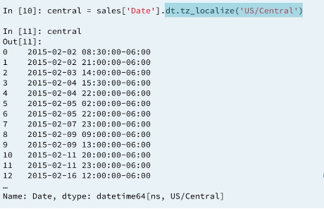
These two operation can be performed at once using method chaining.

3.7 World population

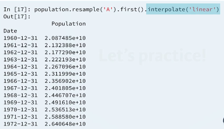
the final manipulation will see here is how to interpolate values.

3.8 Unsample population

For Understanding Manipulating pandas time series

3.9 Interpolation Missing data

For Understanding Manipulating pandas time series

Example 5: Method chaining and filtering

We've seen that pandas supports method chaining. This technique can be very powerful when cleaning and filtering data.

In this exercise, a DataFrame containing flight departure data for a single airline and a single airport for the month of July 2015 has been pre-loaded. Your job is to use .str() filtering and method chaining to generate summary statistics on flight delays each day to Dallas.

INSTRUCTIONS:

• Use .str.strip() to strip extra whitespace from df.columns. Assign the result back to df.columns.
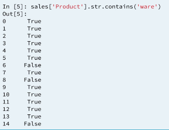
• In the 'Destination Airport' column, extract all entries where Dallas ('DAL') is the destination airport. Use .str.contains('DAL') for this and store the result in dallas.
• Resample dallas such that you get the total number of departures each day. Store the result in daily_departures.
• Generate summary statistics for daily Dallas departures using .describe(). Store the result in stats.

# Strip extra whitespace from the column names: df.columns
df.columns = df.columns.str.strip()

# Extract data for which the destination airport is Dallas: dallas
dallas = df['Destination Airport'].str.contains('DAL')

# Compute the total number of Dallas departures each day: daily_departures
daily_departures = dallas.resample('D').sum()

# Generate the summary statistics for daily Dallas departures: stats
stats = daily_departures.describe()

Example 6 : Missing values and interpolation

One common application of interpolation in data analysis is to fill in missing data.

In this exercise, noisy measured data that has some dropped or otherwise missing values has been loaded. The goal is to compare two time series, and then look at summary statistics of the differences. The problem is that one of the data sets is missing data at some of the times. The pre-loaded data ts1 has value for all times, yet the data set ts2 does not: it is missing data for the weekends.

Your job is to first interpolate to fill in the data for all days. Then, compute the differences between the two data sets, now that they both have full support for all times. Finally, generate the summary statistics that describe the distribution of differences.

Instructions:

• Replace the index of ts2 with that of ts1, and then fill in the missing values of ts2 by using .interpolate(how='linear'). Save the result as ts2_interp`.
• Compute the difference between ts1 and ts2_interp. Take the absolute value of the difference with np.abs(), and assign the result to differences.
• Generate and print summary statistics of the differences with .describe() and print().

# Reset the index of ts2 to ts1, and then use linear interpolation to fill in the NaNs: ts2_interp
ts2_interp = ts2.reindex(ts1.index).interpolate(how='linear')

# Compute the absolute difference of ts1 and ts2_interp: differences 
differences = np.abs(ts1-ts2_interp)

# Generate and print summary statistics of the differences
print(differences.describe())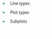

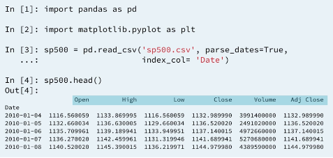
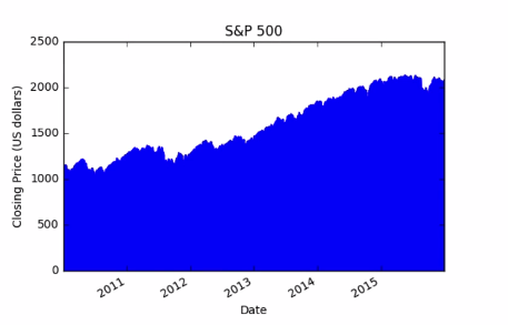
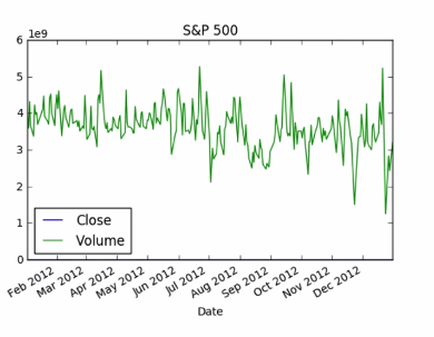
4 Time series visualization

4.1 Topics

4.2 S&P 500 Data

4.3 Pandas plot

4.4 Default plot

4.5 Labels and title

4.5.1 One week

4.6 Plot styles

4.6.1 One week

4.7 more plot styles

4.8 Area plot

4.9 multiple columns

There is a problem with this plot. the volume is so much larger than the price that we can't see the later at this scale. rather using the algorithmic scale lets make separate plot for close price and volume.

4.10 Subplots

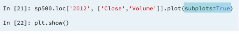
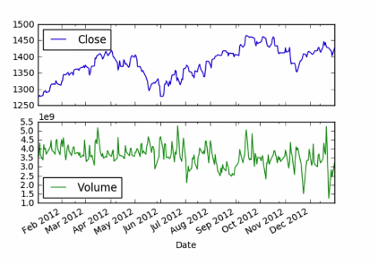
By using subplots=True we can now directly compare assignations between the volume of trade and the closing price.

Example 7: Plotting time series, datetime indexing

Plotting time series, datetime indexing

Example 8 : Plotting date ranges, partial indexing

Plotting date ranges, partial indexing