Repository navigation
Home
An open-source solver for wind-driven rain based on OpenFOAM
Dr. Aytaç Kubilay, Email: akubilay@ethz.ch
Table of Contents:
The source code for the wind-driven rain solver windDrivenRainFoam can be accessed at the following address:
https://github.com/OpenFOAM-BuildingPhysics/windDrivenRainFoam
The following documentation assumes that the user has a working OpenFOAM installation on a Linux system and a basic understanding of how it works. For a list of alternative ways to install OpenFOAM on other operating systems or on a virtual machine, as well as the official user guide, please refer to:
https://www.openfoam.org/
In order to use windDrivenRainFoam, one must go into the downloaded folder that includes the source code:
cd /path/to/windDrivenRainFoam
and compile it by typing:
wmake
The Github repository mentioned above also includes a tutorial case available for download, which models the WDR exposure of an isolated cubic building. Wind-driven rain is modeled so that the rain phase calculations are one-way coupled with the air phase, ignoring the effect of raindrops on the wind flow. Therefore, the tutorial includes two separate case folders, which can be solved consecutively:
- cubicBuilding.simpleFoam and
- cubicBuilding.windDrivenRainFoam.
The former is a typical OpenFOAM case for the simpleFoam solver, which comes with the standard OpenFOAM package and can be used to model incompressible turbulent wind flow with steady Reynolds-averaged Navier-Stokes (RANS). The latter is the solver for the continuity and momentum equations of rain droplets using the calculated wind-flow field as an input. The solver has been validated against field measurements of wind-driven rain on different building configurations and during different rainfall characteristics (Kubilay et al. 2013, 2014, 2015).
The following directories and files exist in a typical OpenFOAM case folder. Depending on the solvers and utilities used, the file structure can be slightly different and/or additional files can be required.
-
0/: This is the initial time directory, which includes the files for the field variables that are used by the solver. Field variables can have scalar, vector, and tensor values. They are named depending on where they are defined in the mesh, e.g. volVectorField for a vector field defined at cell centers, surfaceScalarField for a scalar field defined at face centers of a given grid cell. The files in the 0/ directory include the initial conditions and boundary conditions for the field variables. New time directories are written as the solver runs depending on the output frequency set by the user.
-
constant/polyMesh/: Includes the mesh files.
-
system/: The files located here define the solver settings.
- controlDict: Settings such as timesteps, output frequency, precision, etc.
- fvSchemes: Discretization schemes for each term in the equations are given here.
- fvSolution: Linear solver settings, convergence criteria, under-relaxation, etc.
To begin, one must go into the folder of cubicBuilding.simpleFoam:
cd /path/to/cubicBuilding.simpleFoam
In the tutorial case, mesh is generated using blockMesh utility, which generates a structured hexahedral mesh based on the instructions in file "constant/polyMesh/blockMeshDict". In order to generate the mesh, type:
blockMesh
which will create the computational grid around the cubic building with 10 m height. Mesh files are written under "constant/polyMesh/". Once the mesh is generated and the boundary conditions are specified, wind flow is computed by executing:
simpleFoam
Note that, for simplicity, this manual is written for serial calculation. For parallel computation, please refer to OpenFOAM documentation. The resulting wind-flow field, indicating the acceleration around the building edges and the separation zones, is shown in Fig. 1.
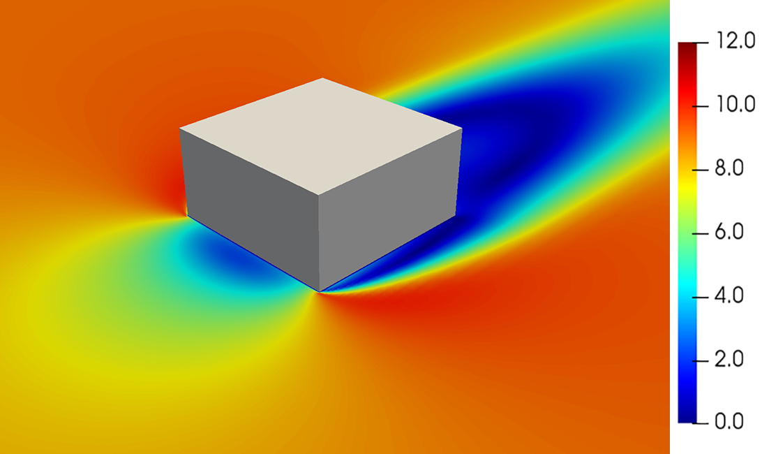
Fig. 1. Magnitude of wind velocity [m/s] at 5 m height.
Depending on the modeling requirements and complexity, different steps can be taken to generate computational grid and to solve wind-flow field. However, this is not within the scope of the present document.
The case folder structure for windDrivenRainFoam is similar to the one for simpleFoam with a few differences. First, the field variables required under time folder 0/ are a list of numbered alpha# and U# fields. These files denote the phase fractions and phase velocities for each separate rain phase. The corresponding raindrop diameter for each rain phase is listed in the file "constant/transportProperties" under a list named "phases" as follows in an increasing order of their size:
phases
(
    0.0003
    0.0004
    ...
    0.005
    0.006
)
where the diameters are given in meters. The file "transportProperties" includes a list of 17 raindrop sizes with diameters ranging from 0.3 to 1 mm in steps of 0.1 mm, from 1 to 2 mm in steps of 0.2 mm and from 2 to 6 mm in steps of 1 mm. Therefore, there are 17 files of U# and alpha# provided under folder 0/. Based on the values given in the list "phases", U1 and alpha1 files are for raindrop diameter of 0.3 mm, U2 and alpha2 for 0.4 mm, etc.
The probability values of different raindrop sizes are calculated for each rainfall intensity [mm/h] given in the list "Rh" based on the probability distribution by Best (1950). This calculation is performed in solver code file "calculateFhD.H". Note that the probabilities are calculated for a range raindrop sizes, e.g. d = 1 mm denotes in fact the raindrop sizes between 0.95 mm and 1.1 mm according to the raindrop size list "phases".
In addition to the list of raindrop sizes, transportProperties file also includes a Boolean variable whether to model turbulent dispersion of raindrops or not (solveTD), a scaling factor for wind-flow field (scalingFactor) and temperature (temp). Note that the wind-flow field is solved for a single reference wind speed in part B. The scaling factor is used to scale wind-flow field for other values of reference wind speed in order to save valuable calculation time. Such scaling is based on the assumption that, for flows around sharp-edged bluff bodies, the positions of flow separation are independent of the Reynolds number. The temperature value is used to calculate air density, air viscosity and raindrop density.
The file "constant/g" denotes the vector of gravitational acceleration. In cases, where the vertical direction is defined different, this file should be edited. Note also that the content of files fvSchemes and fvSolution under system/ folder are slightly different from the ones for simpleFoam calculation.
As the computational grids are identical, the first step before the WDR simulation would be to copy the existing mesh files into the case folder for WDR simulation.
cd /path/to/cubicBuilding.windDrivenRainFoam
cp /path/to/cubicBuilding.simpleFoam/constant/polyMesh ./constant/polyMesh
Once the simpleFoam simulation is complete, the resulting wind velocity field can be copied:
cp /path/to/cubicBuilding.simpleFoam/"lastTime"/U.gz ./0/
If turbulent dispersion of raindrops is modeled, the files for turbulence kinetic energy, k, turbulence dissipation rate, epsilon, and turbulent viscosity, nut, should also be copied in a similar fashion.
For the rain phases, inlet boundaries are defined as the boundaries from which rain enters the computational domain, i.e. the inlet boundary for wind flow as defined in part B for simpleFoam calculation and the top boundary. For these boundaries, the values of rain-phase velocity and rain-phase fraction are defined in each U# and alpha# file under folder 0/.
Boundary condition of rain phase fraction (alpha#) at the inlet and top is of type "fixedValue". Here, a fixed value of 1 is used for the alpha values as below:
inlet
(
	type	fixedValue;
	value	uniform 1.0;
)
top
(
	type	fixedValue;
	value	uniform 1.0;
)
which corresponds to a normalized phase fraction for corresponding raindrop size. If one is interested in the actual phase fraction, this value should be multiplied by the following relation:
where
At the cube walls and ground, boundary condition of type "inletOutlet" is used for the alpha variables. This boundary condition models wall surfaces as outlet in such way that the normal gradient of the phase fraction,
Boundary condition of rain phase velocity (U#) at the inlet is set in such a way that the horizontal component of rain phase velocity has a local force equilibrium between wind flow so that the droplets neither accelerate nor decelerate artificially in an unobstructed computational domain. This is achieved as follows:
- A recycling plane is defined, located downstream of the inlet plane with a certain offset.
- The raindrop velocity profile at the recycling plane is imposed back at the inlet plane.
The inlet/recycling plane couple can also be defined as a “pseudo-periodic condition” at the upstream of the computational domain. This way, the inflow profile for raindrops are generated by itself, which represents a fully-developed rain velocity profile distinct for each separate rain phase. The resulting horizontal component of rain-phase velocity for each different raindrop size will be different as they have different inertia and drag force. This change in the boundary conditions can be performed by typing:
changeDictionary
which uses the instructions in the file "system/changeDictionaryDict", e.g. boundary name, offset of the recycling plane. As an example, Fig. 2a shows the resulting velocity profiles at the inlet for droplets with different diameter. The smallest droplets have a similar profile to the imposed wind profile at the inlet, except for the non-zero velocity on the ground, while larger droplets have a considerably different velocity around the building height due to their larger inertia.
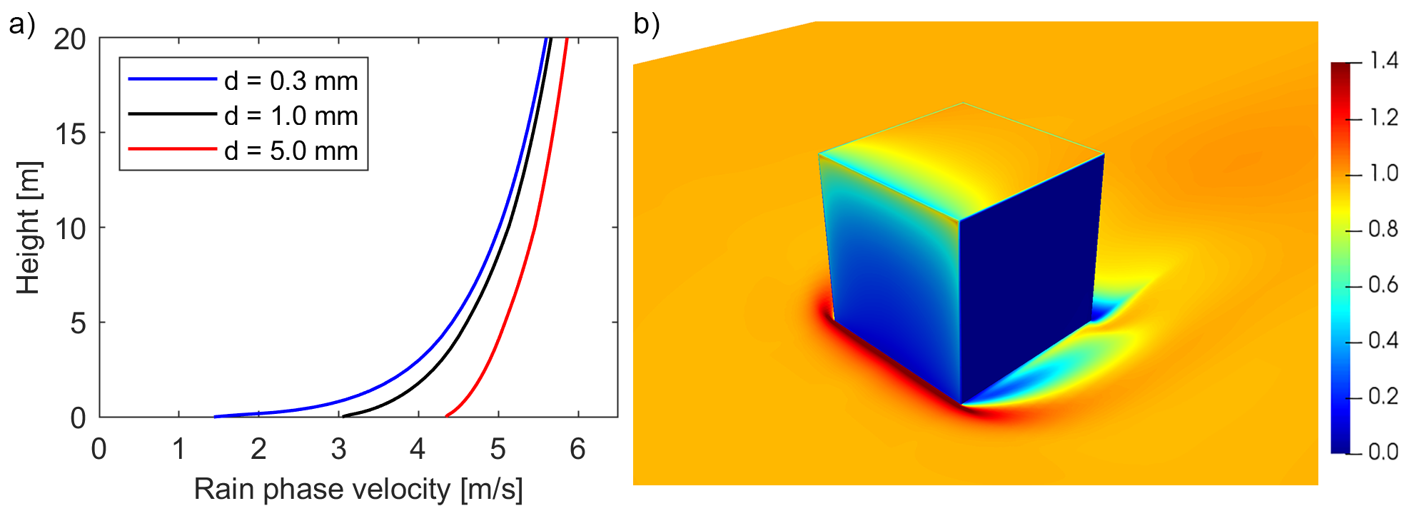
Fig. 2. Streamwise velocity profile at the inlet for droplets with different size and b) the resulting catch ratio [-] distribution on the building surfaces and the surroundings at a rainfall intensity of 1 mm/h and a reference wind speed of 5 m/s.
Note that the same approach is also followed for the boundary condition at the top boundary. The resulting vertical rain phase velocity would be equal to the terminal velocity for that phase, governed by the drag coefficients included in the source code.
The solver (in serial calculation mode) can be run by executing:
windDrivenRainFoam
Once the solver stops (either when it reaches convergence, or when the maximum iteration number is reached), the final timestep is written under the case folder. Under the final time folder, in addition to the U# and alpha# files, scr# and gcr# files are also written. scr# files include the specific catch ratio distribution on the entire surface of the computational domain and defined for each raindrop size in the list "phases" in file constant/transportProperties, e.g. scr1 is for the first raindrop size, which is 0.3 mm. Specific catch ratios are independent of rainfall intensity. In solver code file "calculateCatchRatio.H", these values are multiplied for the probability of raindrop sizes for each rainfall intensity in the list "Rh" in file constant/transportProperties in order to obtain the (global) catch ratio values (Fig. 2b). gcr# files are the (global) catch ratio for each rainfall intensity, e.g. gcr0.1 is for 0.1 mm/h, gcr1 for 1 mm/h, etc.
The solution can be viewed in ParaView by typing:
paraFoam
In addition to the surface wetting, ParaView can also be used to view raindrop trajectories using the "Stream Tracer" function (Fig. 3).
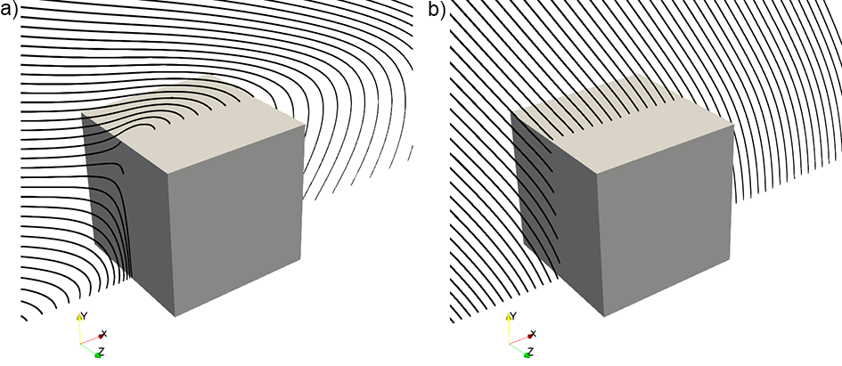
Fig. 3. Trajectories for raindrop sizes of a) 0.5 mm and b) 5 mm at a reference wind speed of 5 m/s.
The necessary steps for windDrivenRainFoam calculation can be summarized as follows:
a. Copy mesh from simpleFoam calculation.
b. Copy the resulting wind-flow field (U, k, epsilon, nut) files from simpleFoam case to the 0/ folder under windDrivenRainFoam case folder.
c. Adjust the scalingFactor by editing the file "constant/transportProperties".
d. Adjust the boundary conditions by running changeDictionary utility.
e. Run solver windDrivenRainFoam.
Best, A.C., 1950. The size distribution of raindrops. Q J Roy. Meteor. Soc. 76, 16–36.
Kubilay, A., Derome, D., Blocken, B., Carmeliet, J., 2013. CFD simulation and validation of wind-driven rain on a building facade with an Eulerian multiphase model. Build. Environ. 61, 69–81.
Kubilay, A., Derome, D., Blocken, B., Carmeliet, J., 2014. Numerical simulations of wind-driven rain on an array of low-rise cubic buildings and validation by field measurements. Build. Environ. 81, 283–295.
Kubilay, A., Derome, D., Blocken, B., Carmeliet, J., 2015. Wind-driven rain on two parallel wide buildings: field measurements and CFD simulations. J Wind Eng. Ind. Aerod. 146, 11–28.