The New Turing Omnibus Chapter 11 Search Trees

Preamble

We welcomed new members to the group and enjoyed home-made scones thanks to Winna and macarons made from Aquafaba thanks to Tom.

The Chapter

We began by talking through the chapter, highlighting some of the potentially confusing terminology (the multiple meanings of "name") but appreciating the two different low-level implementations of search trees.

We discussed the search algorithm described in the text with Chris L stepping through an example on the whiteboard. Paul then offered an alternate, recursive algorithm from Cormen et al's "Introduction to Algorithms" which we translated to fit the book's notation:

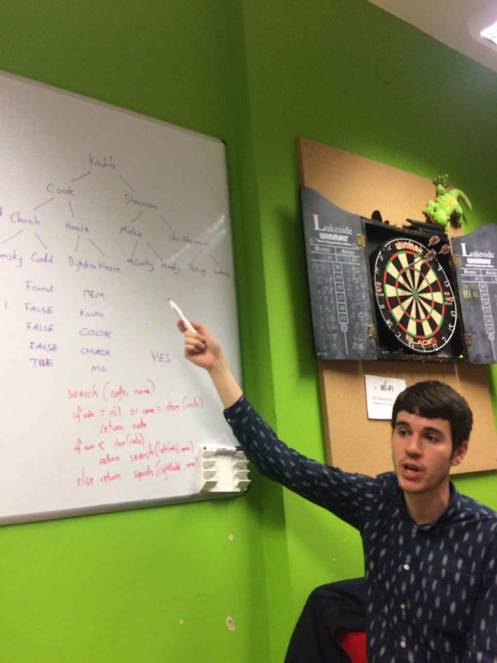
def search(node, name)
  return node if node == nil || name == item(node)

  if name < item(node)
    search(left(node), name)
  else
    search(right(node), name)
  end
end

We then turned to the first exercise in the chapter: what would be the worst shape for a binary search tree?

apple
   \
   banana
     \
     cherry
       \
       durian
         \
         elderberry
           \
           fig

We quickly decided the answer would be a tree (as above) that leans entirely to one side (e.g. with each node to the right of its parent), giving us a worst-case O(n) complexity when searching.

The second part of the exercise asked us to develop an expression for the average complexity (in Big O notation) to search for any item in any arbitrary tree. We were a little confused by this and decided to discuss the best-case complexity given in the chapter in some detail:

There were varying levels of familiarity with Big O notation and computation complexity theory so we attempted a brief summary but felt it might deserve dedicating a future meeting to the topic (particularly as it is a later chapter in the book). We touched on the common complexities:

• O(1): algorithm takes constant time regardless of size of input
• O(n): algorithm grows linearly with the size of input
• O(log n): algorithm grows increasingly slowly with the size of input
• O(n^2): algorithm grows exponentially with the size of input

(We didn't touch on O(n log n).)

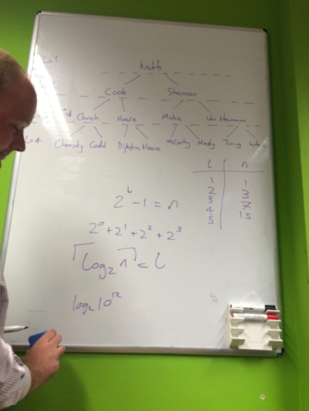
With that in mind, we turned back to the best-case complexity given in the book:

l = ceil(log2 n)

Here, l is the number of levels of the tree and n is the number of nodes in the tree. Given that this only described full, balanced trees, we tried to understand this relationship between levels and nodes and why the ceil is required.

Chris drew up the following table to explore this relationship further and Tom expanded it into the sum of powers in the rightmost column.

number of levels (l)	number of nodes (n)
1	1	20
2	3	20 + 21
3	7	20 + 21 + 22
4	15	20 + 21 + 22 + 23

As this began to take up quite a bit of time (and involved quite a bit of frantic whiteboard action), we decided to move on to the insertion and deletion algorithms.

Insertion was regarded as relatively straightforward as we could use the search algorithm from earlier but modify the last visited node, setting the new node to the left or right appropriately. We worked through this on the whiteboard and then turned to the rather trickier case of deletion.

We worked through a deletion example together on the whiteboard, trying to enumerate the different cases when deleting a node:

1. The node is a leaf (viz. has no left or right subtrees)
2. The node has only one subtree (either the left or right)
3. The node has both left and right subtrees

We talked through the cases and then decided to turn to Jamie's excellent visual implementation to help our understanding.

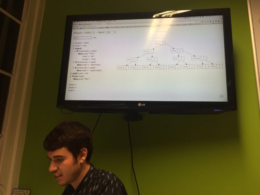
This allowed us to see arbitrary searches, insertions and (some) deletions occurring in real-time, comparing the program's progress with the state of the tree.

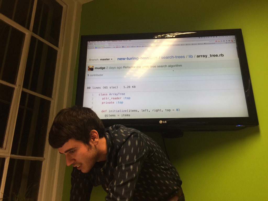
Paul then compared this with his own implementation in Ruby, attempting to use the method described in the book of using three arrays (item, left and right) to store the entire tree.

Paul also discussed an possible immutable version of a tree where insertions and deletions return whole new trees rather than modifying the original. While searching, depth-first and breadth-first ordering were relatively straightforward, the challenge of efficiently returning a new tree on insertion actually requires an exploration of persistent data structures (e.g. techniques such as path copying) which we might revisit in the future.

Feedback

Following the last book's retrospective, we made sure to discuss how the meeting had gone and whether we wanted to make any changes. Overall, the focus on understanding and tying our reading to the specific exercises was a good thing and we were right to be mindful of not overly criticising the material (unless offering a constructive alternative).

As there were clearly many follow-on topics to discuss, we wondered whether to dive deeper into the subject but a good argument was made to explore more varied subjects in future meetings. After all, one of the reasons we chose this book was for its breadth of topics and we wanted to make the club easier to drop in and out of.

Thanks

Thanks to Leo and Geckoboard for hosting, to Jamie for his visual implementation of search trees and to Winna and Tom for sharing their baked goods.