Repository navigation
mexico analysis
This is a knitr document. The source for it contains everything you need to reproduce the analysis given here (aside from the data). The most recent version of this document can always be found at github.com/dill/mexico-data.
The data (which are included in the dsm package) consist of observations of dolphins in the Gulf of Mexico. The analysis is based on a dataset which is shipped with Distance 6.0. For convenience the data are bundled in an R friendly format, although all of the code necessary for creating the data from the Distance project files is available at the above URL.
The intention here is to highlight the features of the dsm package, rather than perform a full analysis of the data. For that reason, some important steps are not fully explored. Some familiarity with density surface modelling is assumed.
Before we start, we load the dsm package and set some options:
library(dsm)## Loading required package: mgcv
## This is mgcv 1.7-22. For overview type 'help("mgcv-package")'.
## Loading required package: mrds
## Loading required package: optimx
## Loading required package: numDeriv
## Loading required package: Rsolnp
## Loading required package: truncnorm
## Loading required package: parallel
## This is mrds 2.1.0 Built: R 2.15.2; ; 2013-01-24 04:04:13 UTC; unix
## Loading required package: ggplot2
## Loading required package: methods
## Loading required package: Distance
## This is dsm 2.0 Built: R 2.15.2; ; 2013-01-28 19:37:37 UTC; unix
# plotting options
gg.opts <- theme(panel.grid.major = element_blank(), panel.grid.minor = element_blank(),
    panel.background = element_blank())
# make the results reproducable
set.seed(11123)All of the data for this analysis has been nicely pre-formatted and is shipped with dsm. Loading up that data, we can see that we have four data frames, the first few lines of each are shown:
data(mexdolphins)
attach(mexdolphins)
head(segdata)
## latitude longitude Effort Transect.Label Sample.Label depth x
## 1 29.94 -86.93 13800 19960417 19960417-1 135.0 134159
## 2 29.84 -86.83 14000 19960417 19960417-2 147.7 143496
## 3 29.75 -86.74 14000 19960417 19960417-3 152.1 152050
## 4 29.66 -86.65 13900 19960417 19960417-4 163.8 161102
## 5 29.56 -86.57 13800 19960417 19960417-5 179.7 169553
## 6 29.49 -86.49 13800 19960417 19960417-6 188.5 176793
## y
## 1 325561
## 2 314055
## 3 304324
## 4 293475
## 5 282984
## 6 275103
head(distdata)## object size distance Effort detected beaufort latitude longitude
## 45 45 21 3296.6 36300 1 4 27.73 -86.00
## 61 61 150 929.2 17800 1 4 26.00 -87.63
## 63 63 125 6051.0 21000 1 2 26.01 -87.95
## 85 85 75 5499.7 21800 1 1 27.50 -90.45
## 114 114 50 7259.0 13400 1 3 27.41 -94.99
## 120 120 45 1454.8 20900 1 5 26.02 -95.97
## x y
## 45 228139 79258
## 61 69199 -113083
## 63 37046 -112197
## 85 -210016 54208
## 114 -658878 43337
## 120 -764824 -111005
head(obsdata)## object Sample.Label size distance Effort
## 45 45 19960421-9 21 3296.6 36300
## 61 61 19960423-7 150 929.2 17800
## 63 63 19960423-9 125 6051.0 21000
## 85 85 19960427-1 75 5499.7 21800
## 114 114 19960430-8 50 7259.0 13400
## 120 120 19960501-5 45 1454.8 20900
head(preddata)## latitude longitude depth x y width height
## 1 30.08 -87.58 35 70832 341079 32072 37065
## 2 30.08 -87.42 30 86868 341079 32072 37065
## 3 30.08 -87.25 27 102904 341079 32072 37065
## 4 30.08 -87.08 22 118940 341079 32072 37065
## 5 30.08 -86.92 46 134976 341079 32072 37065
## 6 29.92 -87.75 14 54888 322546 32126 37065
distdata holds the distance sampling data which will be used to fit the detection function. segdata holds the segment data: the transects have already been "chopped" into segments. obsdata holds the observations which have already been aggregated to the segments and preddata holds the prediction grid (which includes all the covariates that we need).
Typically it will be necessary to pre-allocate the observations to segments (as well as define the segment length) using a tool such as ArcGIS before starting an analysis using dsm.
The below figure shows the survey area with the transect lines overlaid (using data from segdata).
p <- qplot(data = survey.area, x = longitude, y = latitude, geom = "polygon",
    fill = I("lightblue"), ylab = "Latitude", xlab = "Longitude", alpha = I(0.7))
p <- p + coord_equal()
p <- p + gg.opts

p <- p + geom_line(aes(longitude, latitude, group = Transect.Label), data = segdata)

print(p)
It is important to ensure that the measurements to be used in the analysis are in compatible units, otherwise the resulting estimates will be incorrect or hard to interpret. Having all of our measurements in SI units from the outset removes the need for conversion later, making life much easier. All of the data is already in th appropriate units (Northings and Eastings: kilometres from ~-88.32 longitude, ~27.02 latitude, which is the centroid of the study region, multiplyied up by 1000 to get the result in metres for consistency).
It is also important to note that the area of the prediction cells must be included for prediction to work. Our data includes the width and height of each prediction cell and we calculate the areas as needed. See below.
We give an example of converting the survey area here to show that this is a simple process:
# centroid
lon0 <- -88.31951
lat0 <- 27.01594

sa.tmp <- latlong2km(survey.area$longitude, survey.area$latitude, lon0 = lon0,
    lat0 = lat0)

survey.area <- data.frame(x = 1000 * sa.tmp$km.e, y = 1000 * sa.tmp$km.n)

rm(sa.tmp)
The function latlong2km makes this conversion simple (thanks to Simon N. Wood for providing code). The other data frames have already had their measurements appropriately converted. Note that by convention the directions are named x and y.
Using latitude and longitude when performing spatial smoothing can be problematic when certain smoother bases are used. In particular when bivariate isotropic bases are used the non-isotropic nature of latitude and longitude is inconsistent (moving one degree in one direction is not the same as moving one degree in the other).
The top panels of the below figure show histograms of observed distances and group size and the bottom panels show the relationship between observed distance and observed group size, and the relationship between observed distance and Beaufort sea state. The plots show that there is some relationship between size and observed distance to be explored since as one would expect, fewer smaller groups seem to be seen at larger distances.
# save graphics options
o <- par("mfrow")
par(mfrow = c(2, 2))

# histograms
hist(distdata$distance, main = "", xlab = "Distance (m)")
hist(distdata$size, main = "", xlab = "Group size")

# plots of distance vs. size
plot(distdata$distance, distdata$size, main = "", xlab = "Distance (m)", ylab = "Group size",
    pch = 19, cex = 0.5, col = rgb(0.74, 0.74, 0.74, 0.7))

# lm fit
l.dat <- data.frame(distance = seq(0, 8000, len = 1000))
lo <- lm(size ~ distance, data = distdata)
lines(l.dat$distance, as.vector(predict(lo, l.dat)))

plot(distdata$distance, distdata$beaufort, main = "", xlab = "Distance (m)",
    ylab = "Beaufort sea state", pch = 19, cex = 0.5, col = rgb(0.74, 0.74,
        0.74, 0.7))
# restore graphics options
par(o)
## NULL
Looking separately at the at the spatial data without thinking about the distances, we can see the distribution of group size in space in the below figure. Circle size indicates the size of the group in the observation. There are rather large areas with no observations, which might cause our variance estimates to be rather large.
p <- qplot(data = survey.area, x = x, y = y, geom = "polygon", ylab = "y", xlab = "x",
    alpha = I(0.7), fill = I("lightblue"))
p <- p + gg.opts
p <- p + coord_equal()
p <- p + labs(size = "Group size")
p <- p + geom_line(aes(x, y, group = Transect.Label), data = segdata)
p <- p + geom_point(aes(x, y, size = size), data = distdata, colour = "red",
    alpha = I(0.7))
print(p)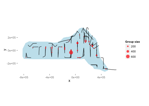
We will use depth later as an explanatory covariate in our spatial model. The next plot shows the raw depth data.
p <- ggplot(preddata)
p <- p + gg.opts
p <- p + coord_equal()
p <- p + labs(fill = "Depth", x = "x", y = "y")
p <- p + geom_tile(aes(x = x, y = y, fill = depth, width = width, height = height))
print(p)
Combining the above two plots yields:
p <- ggplot(preddata)
p <- p + gg.opts
p <- p + coord_equal()
p <- p + labs(fill = "Depth", x = "x", y = "y", size = "Group size")
p <- p + geom_tile(aes(x = x, y = y, fill = depth, width = width, height = height))
p <- p + geom_line(aes(x, y, group = Transect.Label), data = segdata)
p <- p + geom_point(aes(x, y, size = size), data = distdata, colour = "red",
    alpha = I(0.7))
print(p)
This plot shows that we don't seem to have many observations in the very shallow aeas near the shore. This should make us skeptical of predictions in those areas.
We use the ds function in Distance to fit the detection function. First, loading the Distance library:
library(Distance)We can then fit a detection function with hazard-rate key with no adjustment terms:
hr.model <- ds(distdata, max(distdata$distance), key = "hr", adjustment = NULL)## Fitting hazard-rate key function
## AIC= 841.253
## No survey area information supplied, only estimating detection function.
summary(hr.model)##
## Summary for distance analysis
## Number of observations : 47
## Distance range : 0 - 7847
##
## Model : Hazard-rate key function
## AIC : 841.3
##
## Detection function parameters
## Scale Coefficients:
## estimate se
## (Intercept) 7.983 0.9532
##
## Shape parameters:
## estimate se
## (Intercept) 0 0.7835
##
## Estimate SE CV
## Average p 0.5913 0.2224 0.3762
## N in covered region 79.4879 30.8073 0.3876
plot(hr.model)
For brevity, detection function model selection has been omitted here. In practise we would fit many different forms for the detection function, below we fit a detection function with size as a covariate, but for now we stick to a simple model.
Before fitting a dsm model, the data must be segmented; this consists of chopping up the transects and attributing counts to each of the segments. As mentioned above, these data have already been segmented.
We begin with a very simple model. We assume that the number of individuals in each segment are quasi-Poisson distributed and that they are a smooth function of their spatial coordinates (note that the formula is exactly as one would specify to gam in mgcv). The abundance of groups rather than individuals can be estimated by setting group=TRUE (though we ignore this here).
Running the model:
mod1 <- dsm(N ~ s(x, y), hr.model$ddf, segdata, obsdata)
summary(mod1)
##
## Family: quasipoisson
## Link function: log
##
## Formula:
## N ~ s(x, y) + offset(off.set)
## <environment: 0x108e42008>
##
## Parametric coefficients:
## Estimate Std. Error t value Pr(>|t|)
## (Intercept) -18.409 0.394 -46.7 <2e-16 ***
## ---
## Signif. codes: 0 '***' 0.001 '**' 0.01 '*' 0.05 '.' 0.1 ' ' 1
##
## Approximate significance of smooth terms:
## edf Ref.df F p-value
## s(x,y) 26.1 28.2 4.42 4.1e-12 ***
## ---
## Signif. codes: 0 '***' 0.001 '**' 0.01 '*' 0.05 '.' 0.1 ' ' 1
##
## R-sq.(adj) = 0.113 Deviance explained = 44%
## GCV score = 42.985 Scale est. = 37.611 n = 387
We can then make the predictions over the the grid and calculate abundance. First we must create the offset (the area of each grid cell, which is 444km$^2$).
off.set <- 444 * 1000 * 1000
mod1.pred <- predict(mod1, preddata, off.set)
Below is a map of the predicted abundance. Before plotting, we bind on the predicitons to the data used to create them:
pp <- cbind(preddata, mod1.pred)Then plotting:
p <- ggplot(pp) + gg.opts
p <- p + geom_tile(aes(x = x, y = y, fill = mod1.pred, width = width, height = height))
p <- p + coord_equal()
p <- p + geom_path(aes(x = x, y = y), data = survey.area)
p <- p + labs(fill = "Abundance")
print(p)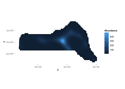
We can calculate abundance over the survey area by simply summing these predictions:
sum(mod1.pred)## [1] 47034
We can also look at diagnostic plots for the model.
gam.check(mod1)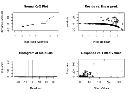
##
## Method: GCV   Optimizer: outer newton
## full convergence after 4 iterations.
## Gradient range [4.281e-07,4.281e-07]
## (score 42.99 & scale 37.61).
## Hessian positive definite, eigenvalue range [0.4516,0.4516].
##
## Basis dimension (k) checking results. Low p-value (k-index<1) may
## indicate that k is too low, especially if edf is close to k'.
##
##           k'   edf k-index p-value
## s(x,y) 29.00 26.06    1.02    0.98
These show that there is some deviation in the Q-Q plot. The "line" of points in the plot of the residuals vs. linear predictor plot corresponds to the zeros in the data.
We can use the approach of Williams et al (2011), which accounts for uncertainty in detection function estimation.
preddata.varprop <- split(preddata, 1:nrow(preddata))
offset.varprop <- as.list(rep(off.set, nrow(preddata)))
mod1.varprop <- dsm.var.prop(mod1, pred.data = preddata.varprop, off.set = offset.varprop)
Calling summary will give some information about uncertainty estimation:
summary(mod1.varprop)## Summary of uncertainty in a density surface model calculated
## by variance propagation.
##
## Quantiles of differences between fitted model and variance model
## Min. 1st Qu. Median Mean 3rd Qu. Max.
## -4.69e-12 -1.57e-13 -1.40e-14 -2.11e-13 4.00e-15 2.70e-13
##
## Approximate asymptotic confidence interval:
## 5% Mean 95%
## 29962 47034 73832
## (Using delta method)
##
##
## Point estimate : 47034
## Standard error : 10966
## Coefficient of variation : 0.2331
We can also make a plot of the CVs:
plot(mod1.varprop, xlab = "Easting", ylab = "Northing")
The data set also contains a depth covariate (which we plotted above). We can include in the model very simply:
mod2 <- dsm(N ~ s(x, y, k = 10) + s(depth, k = 20), hr.model, segdata, obsdata,
    select = TRUE)
summary(mod2)
##
## Family: quasipoisson
## Link function: log
##
## Formula:
## N ~ s(x, y, k = 10) + s(depth, k = 20) + offset(off.set)
## <environment: 0x10981b708>
##
## Parametric coefficients:
## Estimate Std. Error t value Pr(>|t|)
## (Intercept) -18.823 0.734 -25.6 <2e-16 ***
## ---
## Signif. codes: 0 '***' 0.001 '**' 0.01 '*' 0.05 '.' 0.1 ' ' 1
##
## Approximate significance of smooth terms:
## edf Ref.df F p-value
## s(x,y) 3.88 9 2.06 0.00018 ***
## s(depth) 10.52 19 3.15 9.9e-10 ***
## ---
## Signif. codes: 0 '***' 0.001 '**' 0.01 '*' 0.05 '.' 0.1 ' ' 1
##
## R-sq.(adj) = 0.0929 Deviance explained = 34%
## GCV score = 46.27 Scale est. = 42.967 n = 387
By setting the k parameter we specify the largest complexity for that smooth term in the model; as long as this is high enough (i.e. the number in the edf column is not too close to that in the Ref.df column, we can be sure that there is enough flexibility. However, it may sometimes be necessary to set k to be lower than this to limit the influence of (for example) spatial smoothers in the model.
Setting select=TRUE here imposes extra shrinkage terms on each smooth in the model (allowing smooth terms to be removed from the model during fitting, see ?gam for more information). Although this is not particularly useful here, this can be a good way (along with looking at p-values) to perform term selection.
Again we can plot the predictions from this model:
mod2.pred <- predict(mod2, preddata, off.set)
pp <- cbind(preddata, mod2.pred)
p <- ggplot(pp) + gg.opts
p <- p + labs(fill = "Abundance")
p <- p + geom_tile(aes(x = x, y = y, fill = mod2.pred, width = width, height = height))
p <- p + coord_equal()
p <- p + geom_path(aes(x = x, y = y), data = survey.area)
print(p)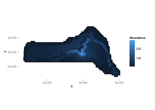
We can also look at the relationship between depth and abundance:
plot(mod2, select = 2)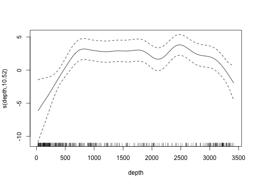
Omitting the argument select gives plots of all the smooth terms, one at a time.
Tweedie
Response distributions other than the quasi-Poisson can be used, for example the Tweedie distribution. If the Tweedie is used, then the p parameter must be specified. Mark Bravington (via personal communication) suggests the use of p=1.2 for marine mammal work. The choice of p is only sensitive to the first decimal place, so a quick search can be performed by simply comparing the score of the resulting models.
mod3 <- dsm(N ~ s(x, y), hr.model, segdata, obsdata, family = Tweedie(p = 1.2))
summary(mod3)
##
## Family: Tweedie(1.2)
## Link function: log
##
## Formula:
## N ~ s(x, y) + offset(off.set)
## <environment: 0x1096543c8>
##
## Parametric coefficients:
## Estimate Std. Error t value Pr(>|t|)
## (Intercept) -18.981 0.405 -46.9 <2e-16 ***
## ---
## Signif. codes: 0 '***' 0.001 '**' 0.01 '*' 0.05 '.' 0.1 ' ' 1
##
## Approximate significance of smooth terms:
## edf Ref.df F p-value
## s(x,y) 27.3 28.7 6.48 <2e-16 ***
## ---
## Signif. codes: 0 '***' 0.001 '**' 0.01 '*' 0.05 '.' 0.1 ' ' 1
##
## R-sq.(adj) = 0.0531 Deviance explained = 47.9%
## GCV score = 23.284 Scale est. = 20.239 n = 387
Note that we have to fully specify the family just as in mgcv.
As well as looking at the GCV/UBRE/REML score of the model to assess the value of p we can also look at a plot of the square root of the absolute value of the residuals versus the fitted values gives the following plot:
plot(sqrt(abs(residuals(mod3))), predict(mod3), xlab = "Square root of the absolute value of the residuals",
    ylab = "Fitted values")
where as setting p=1.7:
mod3 <- dsm(N ~ s(x, y), hr.model, segdata, obsdata, family = Tweedie(p = 1.7))
summary(mod3)
##
## Family: Tweedie(1.7)
## Link function: log
##
## Formula:
## N ~ s(x, y) + offset(off.set)
## <environment: 0x109db7f08>
##
## Parametric coefficients:
## Estimate Std. Error t value Pr(>|t|)
## (Intercept) -24.267 0.671 -36.2 <2e-16 ***
## ---
## Signif. codes: 0 '***' 0.001 '**' 0.01 '*' 0.05 '.' 0.1 ' ' 1
##
## Approximate significance of smooth terms:
## edf Ref.df F p-value
## s(x,y) 28.8 29 14.3 <2e-16 ***
## ---
## Signif. codes: 0 '***' 0.001 '**' 0.01 '*' 0.05 '.' 0.1 ' ' 1
##
## R-sq.(adj) = -9.81 Deviance explained = 53.4%
## GCV score = 9.3865 Scale est. = 8.0932 n = 387
we obtain the following plot, which appears to be much flatter:
plot(sqrt(abs(residuals(mod3))), predict(mod3), xlab = "Square root of the absolute value of the residuals",
    ylab = "Fitted values")
Note also the improvement in GCV score.
In general, a "good" value can be found by simply plotting the above along with the GCV score for the model for values of p between 1.1 and 1.9 and looking for the best GCV and "flattest" plot.
Soap film smoothing
To account for a complex region (e.g. a region that includes peninsulae) we can use the soap film smoother. This is provided by the soap film smoother (see references, below).
In order to use a soap film smoother for the spatial part of the model we must create a set of knots for the smoother to use. This is easily done using the make_soap_grid() function in dsm:
soap.knots <- make.soapgrid(survey.area, c(11, 6))## Warning: the condition has length > 1 and only the first element will be
## used
# knot 11 is not outside but is too close according to soap...
soap.knots <- soap.knots[-11, ]
where the second argument specifies the size of the grid that will be used to create the knots (knots in the grid outside of survey.area are removed).
As we saw in the exploratory analysis, some of the transect lines are outside of the survey area. These will cause the soap film smoother to fail, so we remove them:
x <- segdata$x
y <- segdata$y
onoff <- inSide(x = x, y = y, bnd = survey.area)
## Warning: the condition has length > 1 and only the first element will be
## used
rm(x, y)
segdata <- segdata[onoff, ]
We can run a model with both the depth covariate along with a spatial (soap film) smooth:
mod4 <- dsm(N ~ s(x, y, bs = "so", k = 10, xt = list(bnd = list(survey.area))) +
    s(depth), hr.model, segdata, obsdata, knots = soap.knots)
summary(mod4)
##
## Family: quasipoisson
## Link function: log
##
## Formula:
## N ~ s(x, y, bs = "so", k = 10, xt = list(bnd = list(survey.area))) +
## s(depth) + offset(off.set)
## <environment: 0x123b1d1c0>
##
## Parametric coefficients:
## Estimate Std. Error t value Pr(>|t|)
## (Intercept) -19.40 0.62 -31.3 <2e-16 ***
## ---
## Signif. codes: 0 '***' 0.001 '**' 0.01 '*' 0.05 '.' 0.1 ' ' 1
##
## Approximate significance of smooth terms:
## edf Ref.df F p-value
## s(x,y) 23.05 29.00 2.63 2e-07 ***
## s(depth) 7.08 7.89 2.21 0.027 *
## ---
## Signif. codes: 0 '***' 0.001 '**' 0.01 '*' 0.05 '.' 0.1 ' ' 1
##
## R-sq.(adj) = 0.183 Deviance explained = 45.9%
## GCV score = 45.227 Scale est. = 38.341 n = 365
Not that the k argument now refers to the complexity of the boundary smooth in the soap film and the complexity of the film is controlled by the knots given in the xt argument.
Comparing predictions from the model that included a smooth of depth, we can see that the soap film has prevented some of the extreme values (especially in the lower right corner of the survey area).
mod4.pred <- predict(mod4, preddata, off.set)
pp <- cbind(preddata, mod4.pred)

p <- ggplot(pp) + gg.opts
p <- p + geom_tile(aes(x = x, y = y, fill = mod4.pred, width = width, height = height))
p <- p + coord_equal()
p <- p + geom_path(aes(x = x, y = y), data = survey.area)
p <- p + labs(fill = "Abundance")
print(p)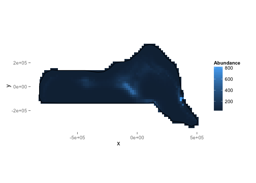
It is common to include covariates in the detection function (so-called Multiple Covariate Distance Sampling or MCDS). In this dataset there is two covariates which are collected on each individual: Beaufort sea state and size. For brevity we fit only a hazard-rate detection functions with the sea state included as a factor covariate as follows:
hr.beau.model <- ds(distdata, max(distdata$distance), formula = ~as.factor(beaufort),
    key = "hr", adjustment = NULL)
summary(hr.beau.model)
##
## Summary for distance analysis
## Number of observations : 47
## Distance range : 0 - 7847
##
## Model : Hazard-rate key function
## AIC : 843.7
##
## Detection function parameters
## Scale Coefficients:
## estimate se
## (Intercept) 7.66318 1.077
## as.factor(beaufort)2 2.27968 17.367
## as.factor(beaufort)3 0.28606 1.019
## as.factor(beaufort)4 0.07174 1.223
## as.factor(beaufort)5 -0.36399 1.537
##
## Shape parameters:
## estimate se
## (Intercept) 0.3004 0.518
##
## Estimate SE CV
## Average p 0.5421 0.1751 0.3229
## N in covered region 86.6957 29.4133 0.3393
Note that we opt to not use adjustments with the covariate model since we cannot ensure that the detection function will remain monotonic if both covariates and adjustment terms are used.
We fit the model as above, simply replacing the detection function model object and changing the response to be Nhat so the abundances are estimated per segment:
mod5 <- dsm(Nhat ~ s(x, y), hr.beau.model, segdata, obsdata)
summary(mod5)
##
## Family: quasipoisson
## Link function: log
##
## Formula:
## Nhat ~ s(x, y) + offset(off.set)
## <environment: 0x11e8d1bc8>
##
## Parametric coefficients:
## Estimate Std. Error t value Pr(>|t|)
## (Intercept) -17.919 0.274 -65.5 <2e-16 ***
## ---
## Signif. codes: 0 '***' 0.001 '**' 0.01 '*' 0.05 '.' 0.1 ' ' 1
##
## Approximate significance of smooth terms:
## edf Ref.df F p-value
## s(x,y) 25.2 27.8 3.6 8.9e-09 ***
## ---
## Signif. codes: 0 '***' 0.001 '**' 0.01 '*' 0.05 '.' 0.1 ' ' 1
##
## R-sq.(adj) = 0.119 Deviance explained = 40.7%
## GCV score = 81.573 Scale est. = 71.124 n = 365
Note that for models where there are covariates at the individual level we cannot calculate the variance via the variance propagation method of Williams et al (2011), but rather must resort to the moving block bootstrap. Other than this, all of the above models can be fitted.
A plot of predicitons from the covariate model:
mod5.pred <- predict(mod5, preddata, off.set)
pp <- cbind(preddata, mod5.pred)

p <- ggplot(pp) + gg.opts
p <- p + geom_tile(aes(x = x, y = y, fill = mod5.pred, width = width, height = height))
p <- p + coord_equal()
p <- p + geom_path(aes(x = x, y = y), data = survey.area)
p <- p + labs(fill = "Abundance")
print(p)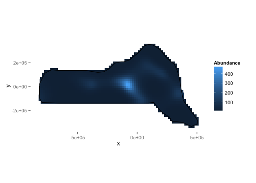
This document has hopefully shown that the dsm package is a versatile and relatively easy-to-use package for the analysis of spatial distance sampling data. Note that there are many possible models that can be fitted using dsm and that the aim here was to show just a few of the options. Results from the models can be rather different, so care must be taken in performing model selection and discrimination.
-
Distanceis available at http://github.com/dill/Distance as well as on CRAN. -
dsmis available (along with some documentation and hints) at http://github.com/dill/dsm, as well as on CRAN.
- Williams, R., Hedley, S.L., Branch, T.A., Bravington, M.V., Zerbini, A.N. & Findlay, K.P. (2011) Chilean Blue Whales as a Case Study to Illustrate Methods to Estimate Abundance and Evaluate Conservation Status of Rare Species. Conservation Biology, 25, 526–535.
- Hedley, S.L. & Buckland, S.T. (2004) Spatial models for line transect sampling. Journal of Agricultural, Biological, and Environmental Statistics, 9, 181–199.