R package for front-end statistical analysis of the EAMENA database
The eamenaR package is under developments. It allows to analyse the typological, spatial and temporal data, to manage data, and to calculate basic statistics (number of HP by grids, users, etc.) from the Arches-powered EAMENA database1. eamenaR is also open to new collaboration2.
flowchart LR
    A[(EAMENA<br>DB)] <--data<br>exchange--> B{{"eamenaR"}}:::eamenaRpkg;
    B --data<br>management--> B;
    B <--data<br>exchange--> C((third part<br>app));
    B --"output"--> D[maps<br>charts<br>listings<br>...];
    classDef eamenaRpkg fill:#e3c071;
The two main sources of data are:
- GeoJSON files exported by EAMENA searches;
- data exported via a direct connection to the EAMENA PostgreSQL database (restricted access);
The two main types of output are:
- static graphs and maps, for publication on paper;
- interactive graphs and maps for publication on the web (with Plotly3 and Leaflet4);
Together with analysis functions, the package offers different methods to manage inputs and outputs from/to EAMENA. The eamenaR package makes the EAMENA DB data FAIR (Findable, Accessible, Interoperable, Reusable)
flowchart LR
    subgraph ide1 [Findable, Accessible]
    A[(EAMENA<br>DB)];
    end
    A[(EAMENA<br>DB)] <---> B{{"eamenaR"}}:::eamenaRpkg;
    subgraph ide2 ["Interoperable, Reusable"]
    B;
    end
    classDef eamenaRpkg fill:#e3c071;
The functions names refer to their content :
| Function prefix | Description | Example |
|---|---|---|
| geojson_* | all functions that deal with GeoJSON | geojson_map() |
| geom_* | any other function that deals with geometries | geom_bbox() |
| list_* | structure a dataset | list_mapping_bu() |
| plot_* | creates a map, a graphic, etc. | plot_edtf() |
| ref_* | direct connection to the EAMENA PostgreSQL database | ref_cultural_periods() |
Correspondances between concept labels and UUIDs
The file ids.csv is a correspondence table between permanent concepts' labels used in this package (r.concept.name), customised concepts' labels used in a specific Arches project db.concept.name and the latter UUIDs db.concept.uuid (by default, these values are those of the reference data/mds). Depending on how you named your Arches instance concepts, you will have to modifiy these correspondences (see the function ref_ids())
| r.concept.name | db.concept.name | db.concept.uuid |
|---|---|---|
| id | EAMENA ID | 34cfe992-c2c0-11ea-9026-02e7594ce0a0 |
| Investigator.Role.Type | Investigator Role Type | d2e1ab96-cc05-11ea-a292-02e7594ce0a0 |
| Geometric.Place.Expression | Geometric Place Expression | 5348cf67-c2c5-11ea-9026-02e7594ce0a0 |
| Cultural.Period | Cultural Period | 3b5c9ac7-5615-3de6-9e2d-4cd7ef7460e4 |
| Cultural.Sub-Period | Cultural Sub-Period | 16cb160e-7b31-4872-b2ca-6305ad311011 |
| Disturbance.Extent.Type | Disturbance Extent Type | 41488800-6c00-30f2-b93f-785e38ab6251 |
Use the Python function
node_uuids()to retrieve the fieldsdb.concept.nameanddb.concept.uuidfor any RM (see documentation)
Install the R package
devtools::install_github("eamena-project/eamenaR")And load the package
library(eamenaR)How it works ?
The root directory on your local computer will be (run): system.file(package = "eamenaR"). By default, output will be saved in the results/ folder. You can change this output folder by changing the dirOut option in the various functions to your choice. The inst/extdata/ folder collects different sample files (GeoJSON, KML/KMZ, XLSX, etc.).
Data will come from two sources: exported files, and SQL queries.
GeoJSON is the preferred format for working with EAMENA. Create a search in EAMENA, in the export menu, copy the geojson url (in green) to the clipboard, paste it into your web browser and create a GeoJSON file.

Paste the copied URL into your web browser and create a GeoJSON file, the result is something like :

You can reformat the (Geo)JSON layout to make it more readable using https://codebeautify.org/jsonviewer. Copy the text content and save it in a new GeoJSON file, for example caravanserail.geojson (rendered | raw).
The PostgreSQL database is queried directly with SQL command passed through a DBI connection (RPostgres::Postgres driver).
Whether the data is Heritage Places, Built Components, etc.
The geojson_stat() function allows to display basic statistics. For example, a pie chart on 'Overall Condition Assessment':
geojson_stat(stat.name = "overall_cond",
             stat = "stats",
             field.names = c("Overall Condition State Type"))

The same chart can be done for an external DB
geojson_stat(geojson.path = "C:/Users/Thomas Huet/Downloads/MAPSS_Xiongnu_khovd.geojson",
             stat.name = "MAPSS_ThreatDriverType",
             stat = "stats",
             field.names = c("Threat Driver Type"),
             export.plot = T,
             dirOut = "C:/Rprojects/eamenaR/results/"
)or an histogram on 'Disturbance Cause Type'
geojson_stat(stat.name = "distrub",
            stat = "stats",
            chart.type = "hist",
            field.names = c("Disturbance Cause Type"),
            fig.width = 10,
            fig.height = 9,
            write.stat = T)

or a radar chart on 'Resource Orientation'
geojson_stat(stat.name = "orientations",
             stat = "stats",
             chart.type = "radar",
             field.names = c("Resource Orientation"),
             fig.width = 9,
             fig.height = 8,
             write.stat = T)

The geojson_boxplot() function creates boxplots. Path lengths, or areas, can be visualized in a boxplot, stratified by a variable (like "route") or not. With areas (stat = area, by default), each dot represents an heritage place. With path lenghts (stat = dist), each dot represent a segment length between two neighbouring caravanserails.
geojson_boxplot(stat = "area")
geojson_boxplot(stat = "dist")


Startified by routes and exported:
geojson_boxplot(stat = "area", by = "route", export.plot = T)
geojson_boxplot(stat = "dist", by = "route", export.plot = T)


In the same way, these boxplot can be made interactive using Plotly, and exported as HTML files
geojson_boxplot(stat.name = "caravanserais_areas", stat = "area", by = "route",
                interactive = T,
                export.plot = T)
geojson_boxplot(stat.name = "caravanserais_dist", stat = "dist", by = "route",
                interactive = T,
                export.plot = T)
See these HTML files, areas and distances
Distribution maps for Heritages places and Geoarchaeology.
The ref_hps() function allows a back-end connection.
Using the default caravanserail.geojson (rendered | raw) Heritage Places GeoJSON file with the geojson_map() function.
geojson_map(map.name = "caravanserail", fig.width = 11, export.plot = T)

Maps can also be calculated on the values of GeoJSON fields, by adding the field names in the geojson_map() function options.
geojson_map(map.name = "caravanserail",
            field.names = c("Damage Extent Type"),
            fig.width = 11,
            export.plot = T)

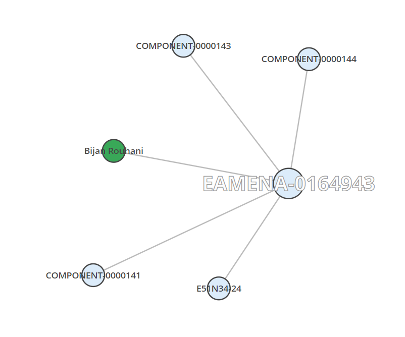
The color of the value (optional) is recorded in the symbology.xlsx file
screenshot of the `symbology.xlsx` file registering the different colors of the values (only the columns `list`, `values` and `colors` are used)
geojson_map(map.name = "caravanserail",
            field.names = c("Disturbance Cause Type ", "Damage Extent Type"),
            fig.width = 11,
            export.plot = T)
It will create two series of maps, one for each field ("Disturbance Cause Type ", "Damage Extent Type") and because in "Damage Extent Type" there are multiple values for a same row, it creates as many maps as there are different values, here is an example:


Finally, Plotly can be used to create an interactive map:
geojson_map(map.name = "caravanserail",
            geojson.path = paste0(exdata, "caravanserail_polygon.geojson"),
            plotly.plot = T,
            export.plot = F)
Will plot this map
Retrieve the matches between these maps' IDs and the EAMENA IDs for heritage places by running the geojson_stat() function:
geojson_stat(stat.name = "caravanserail", stat = "list_ids", export.stat = T)This will give the data frame caravanserail_list_ids.tsv. If you want the maps' IDs listed (e.g. for a figure caption), run :
geojson_stat(stat.name = "caravanserail", stat = "list_ids", export.stat = F)Will give:
1: EAMENA-0192223, 2: EAMENA-0192598, 3: EAMENA-0192599, [...], 153: EAMENA-0194775, 154: EAMENA-0194776, 155: EAMENA-0194777, 156: EAMENA-0194778Reading the GeoJSON file of the heritage places, and the CSV file registering the paths between these heritage places, identified by different routes (route 1, route 2, etc.). Map them using the geojson_map_path() function
geojson_map_path(map.name = "caravanserail_paths", export.plot = T, fig.width = 11)

A good way to control the paths, avoiding double edges, etc. is to run an interactive plot of these paths:
geojson_map_path(interactive = T,
                 export.plot = F)
Will plot these five routes (from 0 to 4) into an interactive VisNetwork HTML widget, for example route 1

Heritages places can be drawn with their elevation, for each route, using two functions: geojson_addZ() to add a their Z value using a geoserver API and the function geojson_map_path() to create the routes profiles (export.type = "profile")
df <- geojson_addZ()
geojson_map_path(geojson.path = "C:/Rprojects/eamenaR/inst/extdata/caravanserailZ.geojson",
                 export.type = "profile",
                 export.plot = T,
                 fig.height = 11,
                 fig.width = 18)

The numbers of the HP are the same as the previous map
The use of POLYGONES (or even LINES), such as caravanserail_polygon.geojson allows to compute shape analysis. For the latter, we use the Momocs functions integrated in the iconr package.
library(Momocs)
library(iconr)

dataDir <- "C:/Rprojects/eamena-arches-dev/projects/caravanserail"
nodes <- conv_geojson_to_wkt(dataDir = dataDir)
conv_wkt_to_jpg(nodes = nodes,
                ids = "site",
                dataDir = dataDir,
                out.dir = "_out")
conv_geojson_to_wkt() and conv_wkt_to_jpg() convert from GeoJSON to JPG, passing through WKT, creating this kind of outputs:


These JPGs are analysed through shape analysis comparisons (here, we limit the study to 50 caravanserails)
dist <- morph_nds_compar(nodes = nodes,
                         cex = .5,
                         lwd = .5,
                         colored = FALSE,
                         dataDir = dataDir,
                         out.dir = "_out")
The variable dist stores the distance matrix between each pairs of caravanserails. The morph_nds_compar() output plots are :

panel

stack

PCA

HCA
After the shape comparisons, a classification can be made with morph_nds_group(). The HCA shows that there are two main groups (or centres, nb.centers = 2). We can reuse this parameter for shape classification:
mbrshp <- morph_nds_group(nodes = nodes,
                          nb.centers = 2,
                          dataDir = dataDir,
                          out.dir = "_out")
It gives a Kmeans plot with 2 centers:

Kmeans with 2 centers
The variable mbrshp stores the membership of all caravanserais (here group 1 or group 2). It can be reused in the geojson_map() function, for example, to locate the different forms of caravanserai.
To manage KML and GeoJSON geometries, the workflow will be to:
flowchart LR
    A[(EAMENA DB)] --search--> A;
    A --export GeoJSON URL--> B[Create GeoJSON file];
    B --import--> C((Google Earth));
    C --"HPs POINTS -> POLYGONS"--> C;
    C --export KML/KMZ--> D{{"geom_kml()"}};
    subgraph eamenaR
    D --"convert KML/KMZ to GeoJSON"--> D;
    D --export--> E{{"geom_bu()"}};
    E --"TODO: format GeoJSON as a BU"--> E
    end
    E --add a new geometry-->A;
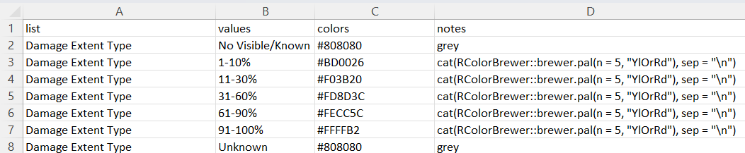
Part of the information of the Heritage Places can be recorded in the Built Components (COMPONENT-), which are connected components of Heritage Places. For example, COMPONENT-0000141, COMPONENT-0000143 and COMPONENT-0000144 record respectively 30 Stables, 1 Courtyard and 28 Rooms for the caravanserail Maranjab (EAMENA-164943).
By default, in EAMENA, relationships between Heritage Places and Built Component are of the type PX_is_related_to, unlike relationships between Heritage Places and Persons (L33_has_maker) or between Heritage Places and Grid Squares (P89_falls_within).
Functions list_related_resources() allows to retrieve this data for a given Heritage Place
d <- hash::hash()
my_con <- RPostgres::dbConnect(drv = RPostgres::Postgres(),
                               user = 'xxx',
                               password = 'xxx',
                               dbname = 'eamena',
                               host = 'ec2-54-155-109-226.eu-west-1.compute.amazonaws.com',
                               port = 5432)

df <- list_related_resources(db.con = my_con,
                             d = d,
                             relationshiptype = "PX_is_related_to",
                             id = "EAMENA-0164943",
                             disconn = FALSE)
df
Will give this df dataframe, with the keys (id and uuid) of the connected components:
| hp.id | hp.uuid | cc.id | cc.uuid |
|---|---|---|---|
| EAMENA-0164943 | d4feb830-10c7-4d80-a19e-e608f424be4c | COMPONENT-0000141 | 90400bb6-ff54-4afd-8183-65c67fa97448 |
| EAMENA-0164943 | d4feb830-10c7-4d80-a19e-e608f424be4c | COMPONENT-0000143 | 0dab164a-6d3a-443c-954a-50d93efbff35 |
| EAMENA-0164943 | d4feb830-10c7-4d80-a19e-e608f424be4c | COMPONENT-0000144 | 28af281c-e4b9-44ac-aa98-2608581b7540 |
Where hp is the Heritage place, and cc the connected component(s). The function select_related_resources() allows to retrieve the values of a given variable. For example, to retrieve the total number of Rooms, use the calculated dataframe df listing the keys (see list_related_resources()) and modify the parameter having. By default the value will be read in the field "Measurement Number" (function parameter measure).
df.measures <- select_related_resources(db.con = my_con,
                                        having = "Room",
                                        df = df)
df.measures
Will give this df.measures dataframe:
| hp.id | hp.uuid | cc.id | cc.uuid | cc.type | cc.measure |
|---|---|---|---|---|---|
| EAMENA-0164943 | d4feb830-10c7-4d80-a19e-e608f424be4c | COMPONENT-0000144 | 28af281c-e4b9-44ac-aa98-2608581b7540 | Room | 28 |
To retrieve the Heritage places' information about Rooms and Stables, create a dataframe to store this data, and run a loop stament over Heritage Places and types of Built components:
hps <- c("EAMENA-0164943", "EAMENA-0164937", "EAMENA-0164905")
bcs <- c("Room", "Stable")

df.measures.all <- data.frame(hp.id = character(),
                              hp.uuid = character(),
                              cc.id = character(),
                              cc.uuid = character(),
                              cc.type = character(),
                              cc.measure = numeric())

for(ea in hps){
  df <- list_related_resources(db.con = my_con,
                               d = d,
                               id = ea,
                               disconn = F)
  for(have in bcs){
    df.measures <- select_related_resources(db.con = my_con,
                                            df = df,
                                            having = have,
                                            disconn = F)
    df.measures.all <- rbind(df.measures.all, df.measures)
  }
}
df.measures.all[ , c("hp.id", "cc.id", "cc.type", "cc.measure")]
Will give:
| hp.id | cc.id | cc.type | cc.measure |
|---|---|---|---|
| EAMENA-0164943 | COMPONENT-0000144 | Room | 28 |
| EAMENA-0164943 | COMPONENT-0000141 | Stable | 30 |
| EAMENA-0164937 | COMPONENT-0000148 | Room | 37 |
| EAMENA-0164937 | COMPONENT-0000149 | Stable | 60 |
| EAMENA-0164905 | COMPONENT-0000145 | Room | 24 |
| EAMENA-0164905 | COMPONENT-0000146 | Stable | 30 |
For MaREA geoarchaeological data, with the geojson_map() function:
geojson_map(map.name = "geoarch",
            ids = "GEOARCH.ID",
            stamen.zoom = 6,
            geojson.path = "C:/Rprojects/eamena-arches-dev/data/geojson/geoarchaeo.geojson",
            export.plot = F)

Either for cultural periods or EDTF formats
Use the ref_cultural_periods() and list_child_concepts() to retrieve the list of cultural periods and subperiods directly from the EAMENA DB.
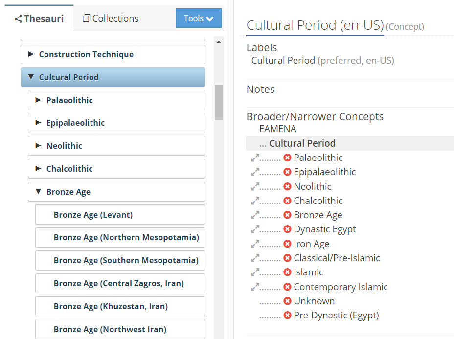
screenshot of the Cultural Periods in the EAMENA Reference Data Manager (RDM)
# create an hash dictionnary to store the cultural ans subcultural periods
d <- hash::hash()
# replace 'xxx' with the username and password
my_con <- RPostgres::dbConnect(drv = RPostgres::Postgres(),
                               user = 'postgres',
                               password = 'postgis',
                               dbname = 'eamena',
                               host = 'ec2-54-155-109-226.eu-west-1.compute.amazonaws.com',
                               port = 5432)
# get cultural periods and subcultural periods
d <- list_child_concepts(db.con = my_con, d = d,
                         field = "cultural_periods",
                         concept.name = 'Cultural Period',
                         disconn = F)
d <- ref_cultural_periods(db.con = my_con, d = d,
                          field = "cultural_periods",
                          disconn = F)
d <- list_child_concepts(db.con = my_con, d = d,
                         field = "cultural_subperiods",
                         concept.name = 'Cultural Sub-Period',
                         disconn = F)
d <- ref_cultural_periods(db.con = my_con, d = d,
                          field = "cultural_subperiods")
# export as TSV
df.periods <- rbind(d$cultural_periods, d$cultural_subperiods)
tout <- paste0("C:/Rprojects/eamena-arches-dev/projects/periodo/cultural_periods.tsv")
write.table(df.periods, tout, sep ="\t", row.names = F)
Gives this TSV dataframe with (sub)cultural periods names, tpq and taq
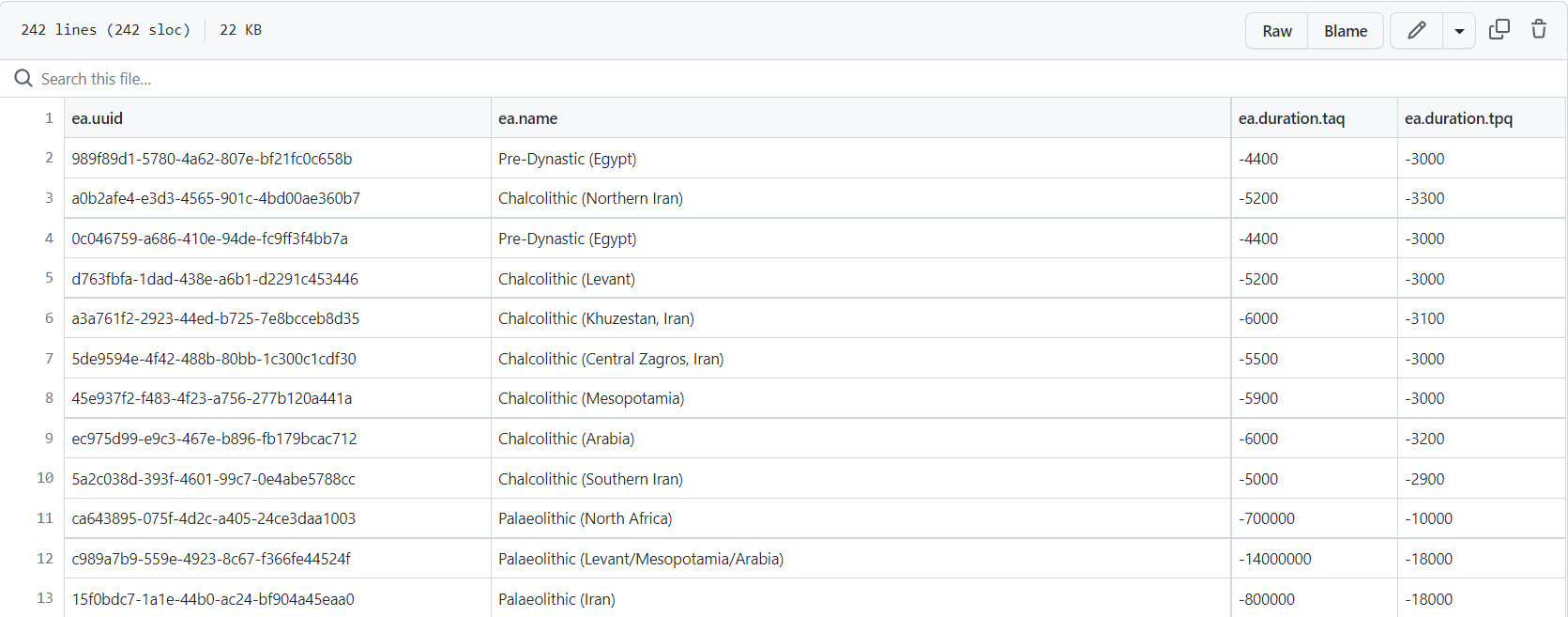
screenshot of the `cultural_periods.tsv` dataframe
How it works ?
These two functions connects the EAMENA DB to parse the arborescence of periods (parents) and superiods (childs) concepts (a tree-like structure) to retrieve their names, their start date (tpq) and end date (taq).
screenshot of the Reference Data Manager, parent node Cultural Period
These latters (start date and end date) are stored in the scopeNote of each cultural periods and subperiods
screenshot of the Reference Data Manager, child node Palaeolithic (Levant/Mesopotamia/Arabia)
Create a hash dictonnary named d to store all data
library(hash)

d <- hash()
Store all periods and sub-periods represented in the GeoJSON in the d dictonnary, and plot them by EAMENA ID using the list_cultural_periods() function
d <- list_cultural_periods(db = "geojson",
                           d = d)
plot_cultural_periods(d = d, field = "periods", plot.type = "by.eamenaid", export.plot = T)
plot_cultural_periods(d = d, field = "subperiods", plot.type = "by.eamenaid", export.plot = T)

and superiods

Here, the plot_cultural_periods() function will export two PNG charts for the default caravanserail.geojson (rendered | raw) file. Periods and subperiods represented in a GeoJSON file can also be summed in a histogram
plot_cultural_periods(d = d, field = "subperiods", plot.type = "histogram", export.plot = T)

Performs an aoristic analysis. By default, the function reads the sample data disturbances_edtf.xlsx and performs the analysis by days (year-month-day: ymd). Two graphs are created, one adding up all the threats, and the other where each category of threat is individualised.
Run the plot_edtf() function with the default parameters.
library(dplyr)

plot_edtf()

Aggregate the dates by months ("ym") by thearts categories.
plot_edtf(edtf_span = "ym", edtf_analyse = "category")

The interactive plotly output is edtf_plotly_category_ym_threats_types.html
Counting and mapping the distribution of Heritage Places created each year using the ref_hps() and plot_hps() functions
# calcualte statistics
stat.name <- "hps_all"
d <- ref_hps(db.con = db.con,
             date.after = '2012-12-31',
             date.before = '2032-12-31',
             d = d,
             stat.name = stat.name)
# create a list of ggplot
lg <- plot_hps(df = d[[stat.name]])
# arrange and save theses plots
margin <- ggplot2::theme(plot.margin = ggplot2::unit(c(.2, -.1, .2, -.1), "cm"))
arranged_plots <- gridExtra::arrangeGrob(grobs = lapply(lg, "+", margin),
                                         ncol = 2)
final_plot <- gridExtra::grid.arrange(
  arranged_plots,
  top = grid::textGrob("Heritage places in the EAMENA database by years",
                       gp = grid::gpar(fontsize = 20, fontface = "bold")),
  bottom = grid::textGrob(paste0("n = ", nrow(sf_df)),
                          gp = grid::gpar(fontsize = 16))
)
ggplot2::ggsave(
  file = "C:/Rprojects/eamenaR/results/hps_by_years.png",
  plot = final_plot,
  height = 19, width = 14
)
Gives:

The function ref_hps() allows to sum the number of HP by GS.
d <- hash::hash()
d <- ref_hps(db.con = my_con,
             d = d,
             stat.name = "eamena_hps_by_grids",
             export.data = TRUE,
             dirOut = 'C:/Rprojects/eamena-arches-dev/data/grids/')
The result is:
- a dataframe listing the number of Heritage Places by GS (first lines):
head(d$grid_nb)| nb_hp | gs |
|---|---|
| 1 | E35N32-14 |
| 635 | E35N32-14 |
| 101 | E51N25-34 |
| 12 | E65N31-13 |
| 17 | E65N31-14 |
| 5 | E64N31-33 |
- an
sffile listing the geometris and UUID of the GS
head(d$grid_geom)Simple feature collection with 6 features and 2 fields
Geometry type: POLYGON
Dimension: XY
Bounding box: xmin: -4.25 ymin: 16.5 xmax: 67.75 ymax: 35
Geodetic CRS: WGS 84
gs ri geom
1 E65N30-13 000170e2-44dd-404a-ac9a-74478b90629c POLYGON ((65 30.25, 65 30.5...
2 W04N16-42 00079b54-194c-4739-b7b4-1e5c24110801 POLYGON ((-4.25 16.5, -4.25...
3 E67N34-43 0010b9cb-4e3d-4603-9d94-683ae1b823e9 POLYGON ((67.5 34.75, 67.5 ...
4 E37N29-12 001adec4-9bf3-4512-a0c0-a13d6043b373 POLYGON ((37.25 29, 37.25 2...
5 E10N21-24 001f9bb7-9961-4cbc-92d7-0af4aec680ee POLYGON ((10.75 21.25, 10.7...
6 E37N29-44 0021d687-c534-4827-8cbb-541e06b4be0d POLYGON ((37.75 29.75, 37.7...
See the output in a GIS, here: https://github.com/eamena-project/eamena-arches-dev/tree/main/data/grids#gis
The function ref_db() provides basic statistics on the users of the EAMENA database, for example by plotting the cumulative distribution function of the user first registration:
d <- hash::hash()
db.con <- RPostgres::dbConnect(drv = RPostgres::Postgres(),
                               user = 'xxx',
                               password = 'xxx',
                               dbname = 'eamena',
                               host = 'ec2-54-155-109-226.eu-west-1.compute.amazonaws.com',
                               port = 5432)
d <- ref_db(db.con = db.con,
            d = d,
            date.after = "2020-08-01",
            plot.g = T,
            fig.width = 14)
Here we restrict the plot to dates after 2020-08-01 (option date.after). The option plot.g = T gives this plot:

The total number of users can also be restricted to an interval (options date.after and date.before), for example limiting the count to the year 2022:
d <- ref_db(db.con = my_con,
               stat.name = "users_date_joined_2",
               d = d,
               date.after = "2022-01-01",
               date.before = "2022-12-01",
               plot.g = T,
               export.plot.g = T,
               fig.width = 14)

d$total_users
#   count
# 1   480
The other statistic calculated is the total number of users (minus those who have an account but have never logged in)
Data management concerns data entry (BU, etc.), search of duplicates, etc.
To facilitate systematic survey, using remote sensing (ex: Google Earth), a grid can be divided into several subgrids using the geojson_grid() function
geojson_grid(geojson.path = paste0(system.file(package = "eamenaR"),
                                   "/extdata/E42N30-42.geojson"),
             rows = 8,
             cols = 4)
Creates this GS with the same extent as the input GS (E42N30-42) and divided into 8*4 subgrids numbered from 1 to 16 (E42N30-42_1 ... E42N30-42_16).
screenshot of Google Pro with the subgrids of E42N30-42 (GeoJSON file)
The Bulk upload procedure to map unformatted datasets, append supplementary data to existing records, etc.
Get a BU file (target, see "what is a BU?") from an already structured file (source) with the list_mapping_bu() function. This function uses a mapping file to create the equivalences between the source file and the target file.
flowchart TD
    A[structured file<br><em><b>source</b></em>] ----> B("list_mapping_bu()"):::eamenaRfunction;
    A -. a. get MBR<br>from geometries .-> D("geom_bbox()"):::eamenaRfunction;
    B <--1. uses--> G[mapping file];
    B --2. export--> C[BU file<br><em><b>target</b></em>];
    subgraph ide1 [Geometries];
      direction LR
      D -. b. creates .-> E[mbr.geojson];
      E -. <a href='https://github.com/eamena-project/eamenaR#collect-the-grid-squares'>used to collect<br>grid squares</a> .-> F[(EAMENA DB)];
      F -. export grid squares<br>in a GeoJSON file .-> H[grid_squares.geojson];
    end;
    H -. add the GRID ID .-> G
    classDef eamenaRfunction fill:#e7deca;
functions:
For example, the dataset prepared by Mohamed Kenawi (mk):
ggsheet <- 'https://docs.google.com/spreadsheets/d/1nXgz98mGOySgc0Q2zIeT1RvHGNl4WRq1Fp9m5qB8g8k/edit#gid=1083097625'
list_mapping_bu(bu.path = "C:/Rprojects/eamena-arches-dev/data/bulk/bu/",
                job = "mk",
                verb = T,
                mapping.file = ggsheet,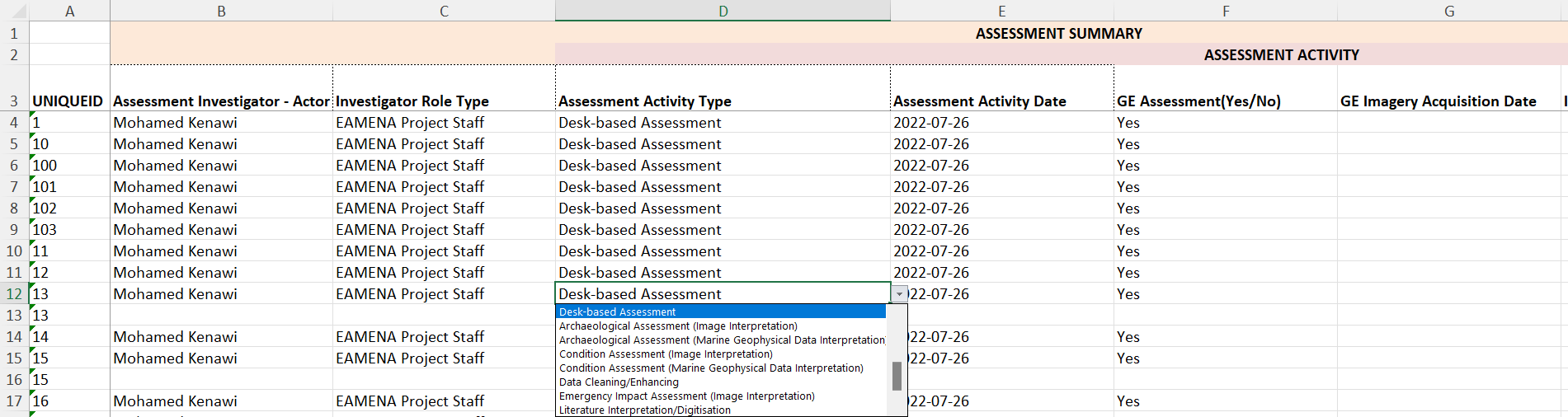
mapping.file.ggsheet = T)To establish the correspondences between a structured file (the source) and the structure of the EAMENA BU template (the target), the list_mapping_bu() function uses a mapping file (ie, a correspondance table). This mapping file could be either an XLSX file or a Google Sheet.
screenshot of the Google sheet mapping file: https://docs.google.com/spreadsheets/d/1nXgz98mGOySgc0Q2zIeT1RvHGNl4WRq1Fp9m5qB8g8k/edit?usp=sharing
For each 'job', the mapping file has three columns, one for the target ('EAMENA', always the same), two for the source (eg. 'mk' and 'mk_type', depending on the job):
- target, by default
EAMENA:
- '
EAMENA': names of the fields in the EAMENA BU template spreadsheet in R format (spaces replaced by dots). Empty cells correspond to expressions that are not directly linked to an EAMENA field. This column will always be the same.
- source:
- The source depends on the different authors:
job: by convention, the initial of the author (e.g. 'mk' = Mohamed Kenawi)job_type: the type of action to perform on the source data (e.g. 'mk_type'). This can be:- '
value': repeat a single value for the whole BU; - '
field': get the different values of a source field and add these different values in a BU field; - '
expression': execute an R code snippet; - '
escape': the value is calculated in another field; - etc.;
- '
The list_mapping_bu() function uses the geom_within_gs() to find the Grid square (gs) identifier of a record by comparing their geometries. By default, the Grid Square file is grid_squares.geojson (rendered | raw)
library(dplyr)

grid.id <- geom_within_gs(resource.wkt = "POINT(0.9 35.8)")
grid.id
Will return "E00N35-44"
Each HP have to be associated with a grid square. If you want to retrieve the grid square ID a posteriori, after you fill the BU - or the BUs - an approriate way to do it is to run the geom_bbox() function.
dataDir <- "C:/Users/Thomas Huet/Downloads/2022-12-08-20221208T154207Z-001/2022-12-08/"

geom_bbox(dataDir = dataDir,
          dirOut = dataDir,
          wkt_column = "Point")
This function retrieve the xmin, xmax, ymin, ymax (minimum bounding box, or MBR) of the HPs and creates as a GeoJSON file, by default: mbr.geojson, like this:
{
    "type": "FeatureCollection",
    "features": [
        {
            "type": "Feature",
            "properties": {
                "buffer": {
                    "width": "0",
                    "unit": "m"
                },
                "inverted": false
            },
            "geometry": {
                "type": "Polygon",
                "coordinates": [
                    [
                        [
                            1.69683243400041,
                            36.4166328242747
                        ],
                        [
                            8.05870602835295,
                            36.4166328242747
                        ],
                        [
                            8.05870602835295,
                            37.0812995946245
                        ],
                        [
                            1.69683243400041,
                            37.0812995946245
                        ],
                        [
                            1.69683243400041,
                            36.4166328242747
                        ]
                    ]
                ]
            }
        }
    ]
}
Copy/paste this mbr.geojson into the EAMENA DB map filter, to select and export the GeoJSON file of grid squares. In EAMENA DB, select Filter > Map Search > Edit GeoJSON and copy/paste the content of the new exported GeoJSON file into the EAMENA Edit GeoJSON field. Under the Search bar, filter by resources (Resource Type) and select Grid Square. Once the filters Map Filtered Enabled and Grid Square are on, only the needed Grid squares appear in the results.
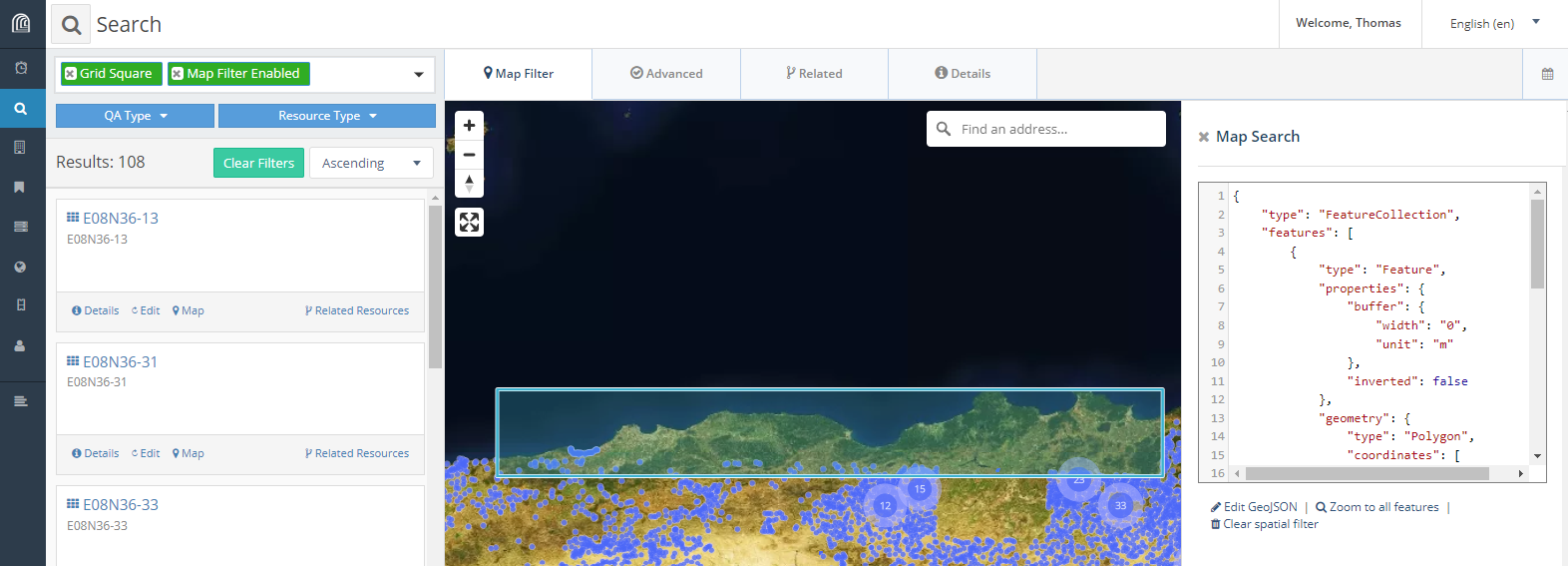
screenshot of the grid squares selection, export them as a new GeoJSON file
Export these grid squares as a geojson url, paste this URL into a web browser, copy the content of the output into a new GeoJSON file5 and save this file. This last GeoJSON file will be used in the geom_within_gs() function to retrieve the correct Grid square ID for each heritage place in the BU.
The source file, or original dataset, is assumed to be an XLSX file but it is possible to work with a SHP, or any other suitable format.
Export a new BU worksheet.
screenshot of the output BU
The data from this new worksheet can be copied/pasted into a BU template to retrieve the drop down menus and 3-lines headers. Once done, the BU can be sent to EAMENA.
screenshot of the output BU once copied/pasted into the template
Append data to existing records (Bulk Upload append).
Using this data to append to the HP 'EAMENA-0188039'
| ResourceID | General.Description.Type | General.Description |
|---|---|---|
| a882affc-60cb-4dcb-a26c-c2721fd0797c | General Description | lorem ipsum |
Where 'a882affc-60cb-4dcb-a26c-c2721fd0797c' is the UUID of 'EAMENA-0188039' (see it in the DB)
Then (in the back-end) run:
python manage.py packages -o import_business_data -s "bu_append_hp_ir_descript.csv" -c "Heritage Place.mapping" -ow appendWill add 'lorem ipsum' to the General Description
A list of related Information Resources (IR) can be append to existing Heritage Places (HP)
| RESOURCEID_FROM | RESOURCEID_TO | START_DATE | END_DATE | RELATION_TYPE | NOTES |
|---|---|---|---|---|---|
| EAMENA-0188039 | INFORMATION-0000052 | x | x | Heritage Resource - Information Resource | x |
| EAMENA-0188041 | INFORMATION-0000052 | x | x | Heritage Resource - Information Resource | x |
| EAMENA-0188042 | INFORMATION-0000052 | x | x | Heritage Resource - Information Resource | x |
| EAMENA-0188043 | INFORMATION-0000052 | x | x | Heritage Resource - Information Resource | x |
see: information_resources_list.csv
This list records relations between HP and IR. Before running a BU append -- that will update the HP adding relations to IR -- it is worth to test if every listed HP already exists in the DB (it also can be done for IR). For example, listing the correspondances between ID (id) and UUID (uuid) using the uuid_id() function:
d <- hash::hash()
bu.to.append <- "https://raw.githubusercontent.com/eamena-project/eamenaR/main/inst/extdata/information_resources_list.csv"
df <- openxlsx::read.xlsx(bu.to.append)
for(i in df[ , "RESOURCEID_FROM"]){
  d <- uuid_id(db.con = my_con,
               d = d,
               id = i,
               disconn = FALSE,
               verbose = FALSE)
  print(paste0(i, " <-> ", d$uuid))
}
Where my_con is a Postgres DB connector. The results
[1] "EAMENA-0188039 <-> a882affc-60cb-4dcb-a26c-c2721fd0797c"
[1] "EAMENA-0188041 <-> b3caf74d-8867-4cde-94fc-0d973c9a0442"
[1] "EAMENA-0188042 <-> d74faf0e-9a66-42c1-b4da-ed0aa5eb3052"
...
If a NA value occurs, in the place of a uuid, it means that the listed HP doesn't exists in the DB.
Most of the geometries in EAMENA are POINTS (Geometry Type = Center Point). The objective is to acquire new geometries, like POLYGONs, created in third part app, like Google Earth or a GIS, and to append them to already existing records in EAMENA.
flowchart LR
    A[(EAMENA<br>DB)] --1. GeoJSON<br><b>POINT</b>--> C("geojson_kml()"):::eamenaRfunction;
    C --2. KML/KMZ--> B((Google<br>Earth));
    B --3. create<br><b>POLYGON</b>--> B;
    B --4. KML/KMZ--> C;
    C --5. GeoJSON<br><b>POLYGON</b>--> D("list_mapping_bu_append()"):::eamenaRfunction;
    D --6. append<br>new geometries--> A;
    classDef eamenaRfunction fill:#e7deca;
workflow to work with Google Earth
flowchart LR
    A[(EAMENA<br>DB)] --1. GeoJSON<br><b>POINT</b>--> E("geojson_shp()"):::eamenaRfunction;
    E --2. SHP--> F((GIS));
    F --3. create<br><b>POLYGON</b>--> F;
    F --4. SHP--> E;
    E --5. GeoJSON<br><b>POLYGON</b>--> D("list_mapping_bu_append()"):::eamenaRfunction;
    D --6. append<br>new geometries--> A;
    classDef eamenaRfunction fill:#e7deca;
workflow to work with a GIS
functions:
For example:
- Export a GeoJSON file from EAMENA (see: GeoJSON files), for example caravanserail.geojson (rendered | raw) Heritage Places.
- Convert caravanserail.geojson to a KML file named 'caravanserail_outKML.kml' with the
geojson_kml()function, filtering on POINTS6:
library(dplyr)
geojson_kml(geom.types = c("POINT"),
            geojson.name = "caravanserail_outKML")
- Open 'caravanserail_outKML' in Google Earth and draw POLYGONS. Name the newly created POLYGONS with the ResourceID of a given HP.

- Export as KML ('caravanserail_outKML2.kml')
- Convert 'caravanserail_outKML2.kml' into GeoJSON with the
geojson_kml()function selecting only the POLYGONs (ie, the new geometries).
geojson_kml(geom.path = geom.path = paste0(system.file(package = "eamenaR"),
                                           "/extdata/caravanserail_outKML2.kml")
            geom.types = c("POLYGON"),
            geojson.name = "caravanserail_outGeoJSON")
The result is new POLYGON geometries (eg. caravanserail_outGeoJSON.geojson)
- Convert the GeoJSON POLYGONs geometries to a format compliant with the EAMENA DB, using the
list_mapping_bu_append()function
list_mapping_bu_append(geom.path = paste0(system.file(package = "eamenaR"),
                               "/extdata/caravanserail_outGeoJSON.geojson"),
            csv.name = "caravanserail_outCSV")
The result is a CSV file, caravanserail_outCSV.csv, with the ResourceID and the geometry of each HP. The fields "Location Certainty" and "Geometry Extent Certainty" are filled with default values.
"resourceid","Geometric Place Expression","Location Certainty","Geometry Extent Certainty"
"8db560d5-d17d-40ff-8046-0157b1b698ab","MULTIPOLYGON (((61.4023 30.77373, 61.4019 30.77371, 61.40194 30.77344, 61.40235 30.77345, 61.4023 30.77373)))","High","High"
"b8305141-789e-4aaa-976a-c85859e0870f","MULTIPOLYGON (((51.47507 33.09169, 51.47463 33.09125, 51.47519 33.09086, 51.47561 33.09133, 51.47507 33.09169)))","High","High"
- These new geometries will be uploaded into the EAMENA DB and append to existing HP having the same
resourceid(ResourceID). But it should be safe to first check that every ResourceID exist in the DB (maybe a newly created POLYGON has a typo in its name). Use theuuid_id()function, in a loop to confirm the existence of the ResourceID
mycsv <- "https://raw.githubusercontent.com/eamena-project/eamenaR/main/inst/extdata/caravanserail_outCSV.csv"
df <- read.csv(mycsv)
for(i in seq(1, nrow(df))){
  eamenaid <- df[i, "ResourceID"]
  d <- uuid_id(db.con = my_con,
                     d = d,
                     id = eamenaid,
                     disconn = FALSE)
  print(paste0(as.character(i), ") ", eamenaid, " <-> ", d$eamenaid))
}
DBI::dbDisconnect(my_con)
Will give:
[1] "1) 8db560d5-d17d-40ff-8046-0157b1b698ab <-> EAMENA-0192281"
[1] "2) b8305141-789e-4aaa-976a-c85859e0870f <-> EAMENA-0182054"
As there are no NA in front of the ResourceID, the HP listed in the CSV file exist in the DB.
- To append these geometries to the DB, use the
-ow appendoption in theimport_business_datafunction (see the Arches documentation)
python manage.py packages -o import_business_data -s "./data/test/caravanserail_outCSV2.csv" -c "./data/test/Heritage Place.mapping" -ow appendNow, each of these two HP has two different kind of geometries: POINT and POLYGON. See for example the whole dataset of caravanserails caravanserail_polygon.geojson, one of the record rendered (EAMENA-0192281.geojson) or this latter record in the EAMENA DB7.
The function ref_are_duplicates() identifies potential duplicates in a GeoJSON file, or directly in the EAMENA database. Using a fuzzy match between the values of a selection of fields, for two HPs identified by their ResourceID, this function creates a data frame with the match score (dist column) between each field:
d <- hash::hash()
d <- ref_are_duplicates(d = d,
                        export.table = T,
                        fileOut = "duplicates.csv")
Creates this kind of table:
| field | 563567f7-eef0-4683-9e88-5e4be2452f80 | fb0a2ef4-023f-4d13-b931-132799bb7a6c | dist |
|---|---|---|---|
| EAMENA ID | EAMENA-0207209 | EAMENA-0182057 | - |
| Assessment.Investigator...Actor | Hamed Rahnama | Hamed Rahnama, Bijan Rouhani | 0.18 |
| Assessment.Activity.Date | 2021-05-25 | 2022-08-21, 2022-08-30 | 0.32 |
| Resource.Name | Bedasht Caravanserai, ..., CVNS-IR | CVNS-IR, Bedasht Caravanserai, ... | 0.26 |
| geometry | c(55.05059, 36.42466) | c(55.05059, 36.42466) | 0 |
The dist shows that the geometries are exactly the same, and that there are slight differences in the other fields. The CSV output is here: https://github.com/eamena-project/eamenaR/blob/main/results/duplicates.csv
Footnotes
-
Arches: https://www.archesproject.org/ ↩
-
https://github.com/eamena-project/eamenaR/blob/main/.github/CONTRIBUTING.md ↩
-
Plotly: https://plotly.com ↩
-
Leaflet: https://leafletjs.com/ ↩
-
You can 'beautify' it using https://codebeautify.org/jsonviewer ↩
-
Sometimes, a search in EAMENA returns different types of geometries. This is the case for the caravanserails where geometries can be both POINTs and POLYGONs. ↩
-
EAMENA-0192281 ResourceID =
8db560d5-d17d-40ff-8046-0157b1b698ab↩