Implementation-of-Logistic-Regression-Using-Gradient-Descent

AIM:

To write a program to implement the the Logistic Regression Using Gradient Descent.

Equipments Required:

1. Hardware – PCs
2. Anaconda – Python 3.7 Installation / Jupyter notebook

Algorithm

1. Use the standard libraries in python for finding linear regression.
2. Set variables for assigning dataset values.
3. Import linear regression from sklearn.
4. Predict the values of array.
5. Calculate the accuracy, confusion and classification report by importing the required modules from sklearn.

Program:

Program to implement the the Logistic Regression Using Gradient Descent.
Developed by: Jayabharathi M
RegisterNumber:  212220220017

import numpy as np
import matplotlib.pyplot as plt
from scipy import optimize
data = np.loadtxt("/content/ex2data1 (2).txt", delimiter=',')
x = data[:, [0,1]]
y = data[:, 2]

print("Array value of x:")
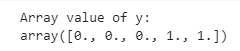
x[:5]

print("Array value of y:")
y[:5]

print("Exam 1-score graph:")
plt.figure()
plt.scatter(x[y == 1][:,0], x[y == 1][:, 1], label="Admitted")
plt.scatter(x[y == 0][:,0], x[y == 0][:, 1], label="Not Admitted")
plt.xlabel("Exam 1 score")
plt.ylabel("Exam 2 score")
plt.legend()
plt.show()

def sigmoid(z):
    return 1 / (1 + np.exp(-z))

print("Sigmoid function graph: ")
plt.plot()
x_plot = np.linspace(-10, 10, 100)
plt.plot(x_plot, sigmoid(x_plot))
plt.show()

def costFunction(theta, x, y):
    h = sigmoid(np.dot(x, theta))
    J = -(np.dot(y, np.log(h)) + np.dot(1 - y, np.log(1 - h))) / x.shape[0]
    grad = np.dot(x.T, h - y) / x.shape[0]
    return J, grad 

x_train = np.hstack((np.ones((x.shape[0], 1)), x))
theta = np.array([0, 0, 0])
J,grad = costFunction(theta, x_train, y) 
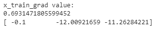
print("x_train_grad value:")
print(J)
print(grad)

x_train  =  np.hstack((np.ones((x.shape[0], 1)), x)) 
theta = np.array([-24, 0.2, 0.2])
J, grad = costFunction(theta, x_train, y)
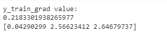
print("y_train_grad value:")
print(J)
print(grad)

def cost(theta, x, y):
    h = sigmoid(np.dot(x, theta))
    J = - (np.dot(y, np.log(h)) + np.dot(1 - y, np.log(1 - h))) / x.shape[0]
    return J

def gradient(theta, x, y):
    h = sigmoid(np.dot(x, theta))
    grad = np.dot(x.T, h - y) / x.shape[0]
    return grad

x_train = np.hstack((np.ones((x.shape[0], 1)), x))
theta = np.array([0, 0, 0])
res = optimize.minimize(fun=cost, x0=theta, args=(x_train, y),
                        method='Newton-CG', jac=gradient)
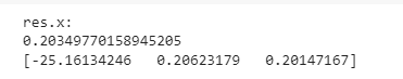
print("res.x:")
print(res.fun)
print(res.x)

def plotDecisionBoundary(theta, x, y):
    x_min, x_max = x[:, 0].min() -1, x[:, 0].max() + 1
    y_min, y_max = x[:, 1].min() -1, x[:, 1].max() + 1
    xx, yy = np.meshgrid(np.arange(x_min, x_max, 0.1),
                         np.arange(y_min, y_max, 0.1))
    x_plot = np.c_[xx.ravel(), yy.ravel()]
    x_plot = np.hstack((np.ones((x_plot.shape[0], 1)), x_plot))
    y_plot = np.dot(x_plot, theta).reshape(xx.shape)
    plt.figure()
    plt.scatter(x[y == 1][:, 0], x[y == 1][:, 1], label="Admitted")
    plt.scatter(x[y == 0][:, 0], x[y == 0][:, 1], label="Not  Admitted")
    plt.contour(xx, yy, y_plot, levels=[0])
    plt.xlabel("Exam 1 score")
    plt.ylabel("Exam 2 score")
    plt.legend()
    plt.show()

print("Descision Boundary - graph for exam score:")
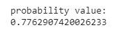
plotDecisionBoundary(res.x, x,y)

print("probability value:")
prob = sigmoid(np.dot(np.array([1, 45, 85]), res.x))
print(prob)

def predict(theta, x):
  x_train = np.hstack((np.ones((x.shape[0], 1)), x))
  prob = sigmoid(np.dot(x_train, theta))
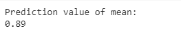
  return (prob >= 0.5).astype(int)

print("Prediction value of mean:")
np.mean(predict(res.x, x)  == y)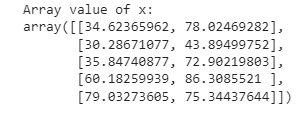

Output:

Result:

Thus the program to implement the the Logistic Regression Using Gradient Descent is written and verified using python programming. Thus the program to implement the the Logistic Regression Using Gradient Descent is written and verified using python programming.