Structured Text Code Clone Detection

This tool analyzes structured text code files and tries to find files which are highly similar. Such highly similar files are called code clones and the associated task of finding such clones is called code clone detection. We implemented different algorithms in this tool in order to find type 3 code clones. Type 3 clones are syntactically similar fragments that differ at the statement level. The fragments have statements added, modified, or removed with respect to each other. Such clones indicate textual and functional similarity [1].

This tool was mainly implemented in Python. At its current state, it comprises 3 analysing approaches: 1. a neural network based algorithm, 2. a principal component analysis (PCA) analysis, and 3. a t-distributed stochastic neighbor embedding (t-SNE) projection. Each of these approaches is explained in detail in the sections below.

Each of these approaches needs a set of token vectors as input. The token vectors are generated out of the structured text code files. More details can be found in the section Architecural Overview.

Installation and Execution

Installation can be performed via docker-compose or via direct execution of the Python files.

Installation via docker-compose

1. Install docker and docker-compose.
2. cd into the directory where the docker-compose file is located.
3. For neural network training, you need to create a data directory in the root directory and fill it with structured text code files.
4. docker-compose up -d --build

Installation via Python

1. Install Python 3.8.
2. Install conda.
3. Create a new conda environment via conda create -n clone_detection python=3.8
4. Run pip install -r requirements.txt
5. Activate the environment conda activate clone_detection
6. Run python main.py

Data Path

An environment variable DATA_PATH must be set. This variable must point to a data folder which contains the structured text files. The generation of the neural network input data requires the data folder to be in a specific format. This format will be explained in the Neural Network section.

Execution

If everything was done correctly, a selection menu with the implemented algorithms appears as shown in the image below. The user can select the desired algorithm from this menu.

Architecural Overview

The following image depicts the workflow of our approach.

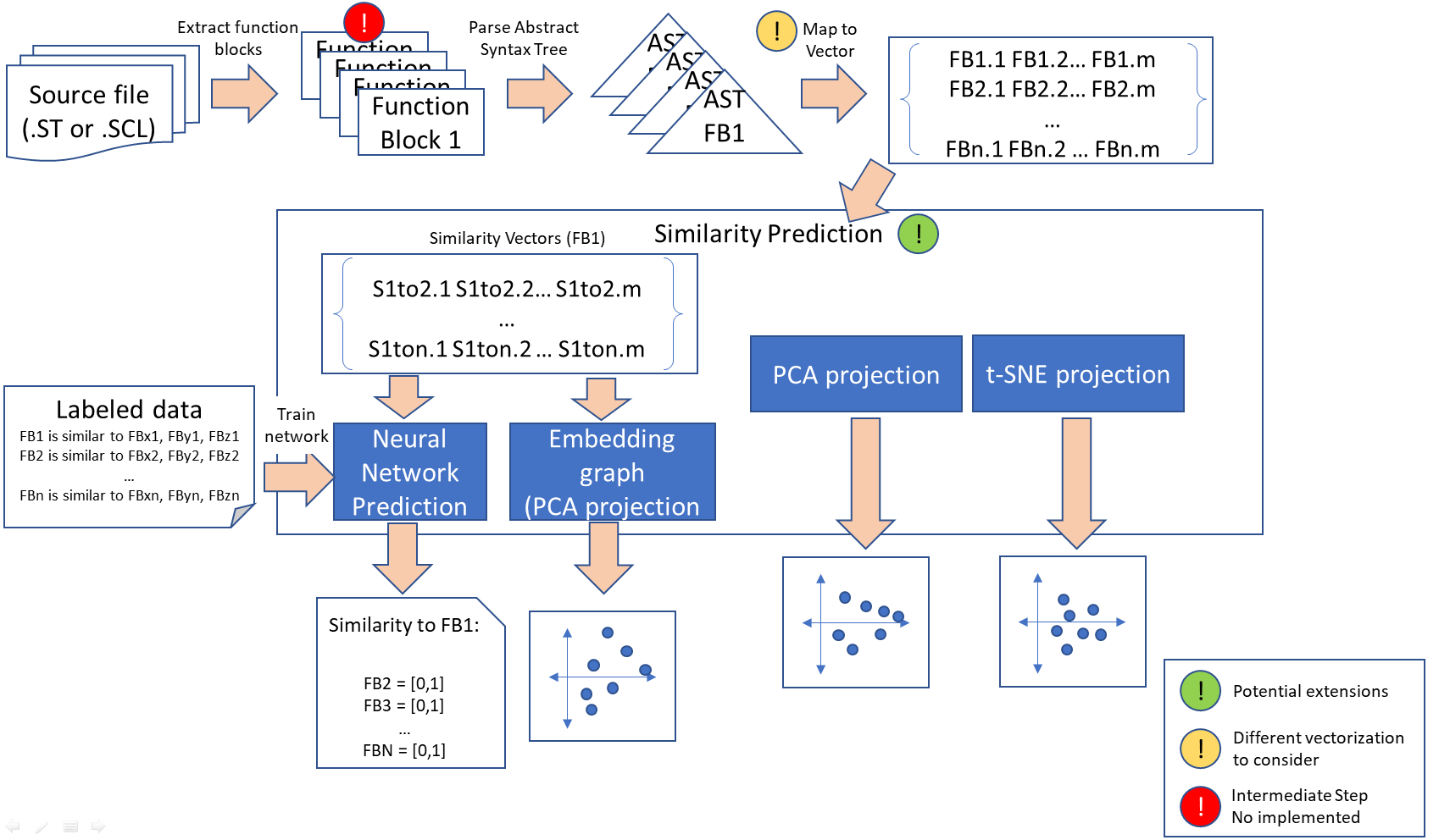
Step 1. Function blocks are extracted from the structured text code files. The extraction was implemented for files with single function blocks. This means that structured text code files with multiple function definitions cannot be analysed yet.

Step 2. Parsing and abstract syntax tree (AST) creation. The extracted functions are parsed for syntactical correctness and subsequently transformed into an AST. We employed pyparsing for the AST creation as it is simple to use and easy to debug grammatical errors.

Step 3: Transformation of extracted symbols into token vectors. This step takes the AST as input and counts the occurrence of individual AST tokens. The result is saved into a Python dictionary whereas the token names are used as keys.

Step 4. Creating similarity vectors. In this step, we create a similarity vector between a pair of token vectors and calculate the similarity with respect to each token. This algorithm is similar to the one described in [2]. The similarity vectors are persisted as numpy binary files using pickle.

Step 5. Performing training and Inference. The similarity vectors are the input to all machine learning algorithms. The unsupervised methods (PCA and t-SNE) perform inference directly on these vectors. The neural network uses the vectors as training data.

Implemented algorithms

1. Neural Network

Data

Since this is a supervised technique, labels are needed in order to be able to perform training. Labels are simple binary: is clone, is no clone. Since no public dataset is available which contains labeled structured code clones (as to our best knowledge), we needed to create training data by ourselves. Hence, we employed a code clone generator which is able to modify the original structured text files slightly in order to obtain code clones. The code clones are very similar to their original counterparts, the modifications comprise mainly the addition and deletion of single line statements. This generator does not take syntactical correctness into account, so we had to delete generated code clones which were not able to be parsed by our parser.

The generated file structure is laid out in the following way:

• data
  • original
    • .st
  • originalandclones
    • clones
      • <modified_filename>.st
  • registry
    • registry.csv
    • <TRAINED_*>.txt

In our implementation, we iterate over the filenames which are located in the original directory. For each filename, we look up a corresponding <TRAINED_FILENAME>.txt file in the registry. These files encode a list of file IDs of clones and non-clones for each of the original files. Each ID can be looked up in the registry.csv file which maps file IDs to files in the originalandclones directory. The clones and non-clones are tokenized and correspoinding labels are created. (1 for is clone and 0 for is not a clone). This way, we were able to generate over 10000 training examples.

Neural Network Architecture

The neural network algorithm employs a feed forward neural network (NN) with 3 layers and ReLU activations in between. Binary Cross Entropy was used as loss function which minimizes the loss between the binary label and the NN output. During inference, a value between 0 and 1 is generated by the NN which can be interpreted as the probability the similarity vector is a clone. The NN was implemented using Pytorch.

Execution

When choosing Neural Network from the main selection menu described above, the tool checks if similarity vectors are available as training data. If not then they need to be generated first, using the training data located by the DATA_PATH environment variable. Next, the network trains for a couple of seconds. As soon as training is finished, a webserver starts which serves a web application. This web application is reachable at http://127.0.0.1:5000/upload/. Entering this URL into the browser opens the following website.

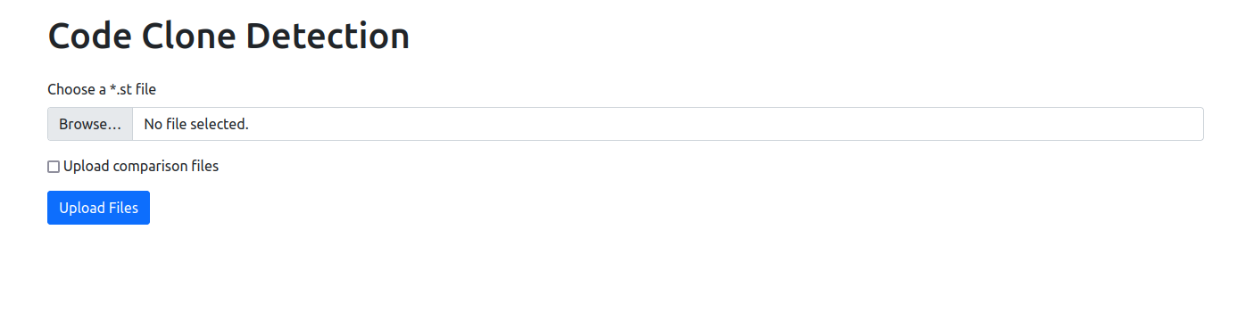
This simple webinterface allows the upload for structured text files which can be compared with all files (called comparison files in the following) located in the original directory. If a file is selected in the file chooser and the upload button is pressed, the uploaded file will be transformed into pairwise similarity vectors. The similarity vectors are fed into the NN. As soon as all files are finished analyzing, the result is shown in the web interface.

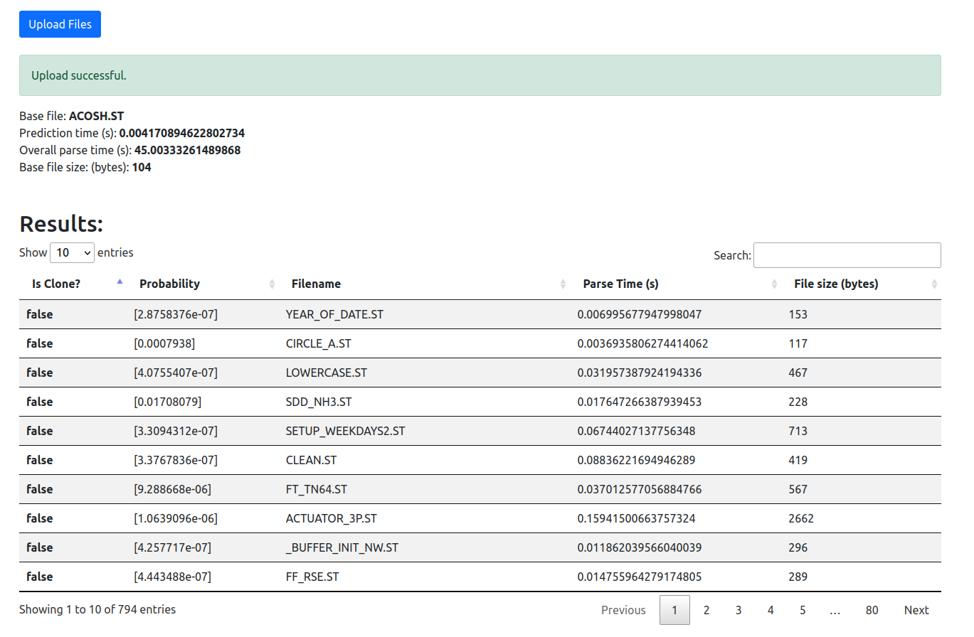
The result is depicted as a paginated table view which is sortable and filterable. Each row depicts a pairwise clone comparision between the uploaded file and the comparision files. The columns of this table are as follows:

1. Is Clone?: Whether it is a clone or not. A binary threshold of 50% was used.
2. Probability: The probability (between 0 and 1) that the comparison file is a clone.
3. Filename: The name of the file
4. Parse time: The time used for parsing

Furthermore, a PCA analysis is performed and depicted below the table view.

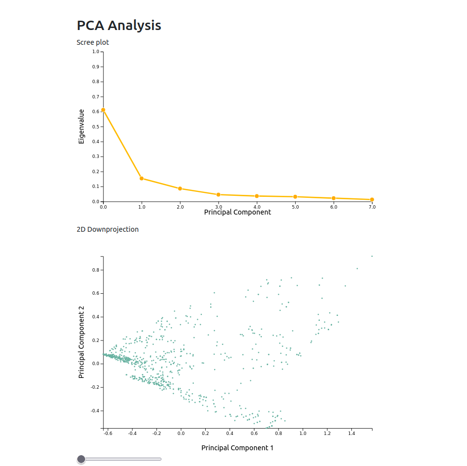
The first linechart shows the explained variance of the principal components. Most often, the first 2-3 principal components explain over 70% of the data variance. The scatter plot below shows the projected data of the first 2 principal components. So each dot in this chart depicts a similarity vector. The slider under this plot acts as a filter. Moving the slider to the right filters file filters similarity vectors that exceed a probability threshold. So the more the slider is moved to the right, the more unprobable code clones are removed from the chart.

2. Principal Component Analysis

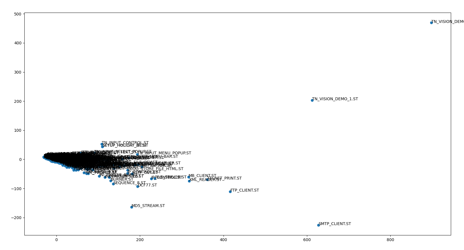
PCA is a dimensionality reduction method that removes features in the data whereas most of the data variance is preserved. As described above PCA is already employed for reducing the dimensionality of the similarity vectors. Further, PCA was implemented to visualize clusters of source files directly. The source files are transformed into token vectors and thereafter, projected onto 2 dimensions. The scatter plot below shows that most of the files are classified as similar. However some outliers exist.

3. t-distributed stochastic neighbor embedding (t-SNE)

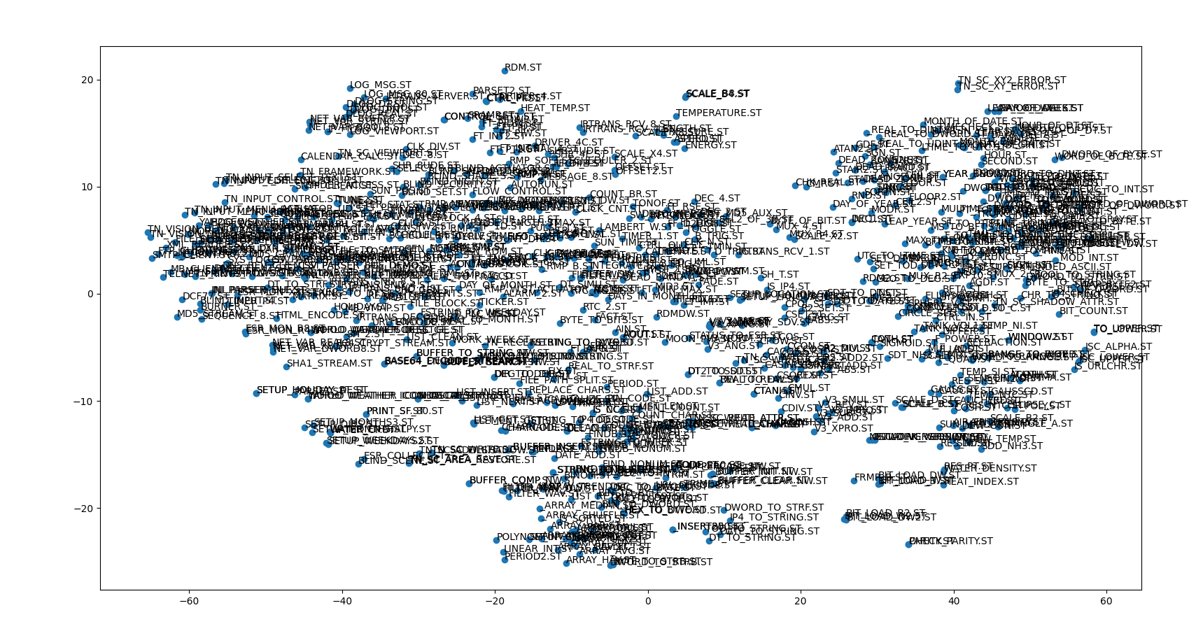
T-SNE is similar to PCA a dimensionality reduction method. Different to PCA, T-SNE is a probabilistic algorithm and assigns a probability value to each pair of objects. The more similar a pair is the highter its probability value. Similar to the PCA implementation, the T-SNE approach takes the original source files and creates token vectors. The token vectors are used as input to the t-SNE algorithm. The output for the same data as in 2. is depicted in the image below. Here it becomes more obvious compared to 2. that some files are more similar and hence potential clones. For example, in the lower right corner is a cluster which comprises of the files BIT_LOAD_B.ST, BIT_LOAD_B2.ST, BIT_LOAD_W.ST, BIT_LOAD_DW.ST and BIT_LOAD_W2.ST. When inspecting these code files, it becomes obvious that they are indeed very similar and hence, can be categorized as clones.

References

[1] Deep Learning Code Fragments for Code Clone Detection, Martin White et. al [2] CCLearner: A Deep Learning-Based Clone Detection Approach, Liuqing Li et. al