Home

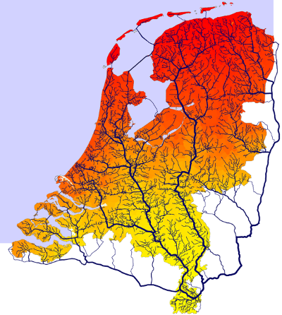
Accessibility in spatial applications is the quality of how easy it is to reach (a) destination location(s).

It is an important driving factor in Land Use Modelling and also relevant for many other applications.

structure of this wiki

• How to find the shortest path between an origin and destination
• Network optimisation algorithms
• What if you want to look at more than one origin and or destination
• How can we use these matrices to say something about accessibility (diving into Spatial Interaction Models)
• Overview of useful Accessibility indicators
• Applications

Finding the shortest path using the Dijkstra Algorithm

The shortest path that has to be found does not necessarily need to be about minimising distance, but it could also be travel time, travel cost, or any metric you could think of. A more general way to think about this is to minimise the impedance of a segment (e.g., a piece of road) in the network. The procedure for finding the shortest path is a large part of graph theory.

The dijkstra algorithm determines the minimum impedance of the routes through a network/graph of nodes and links with given link-impedance for each combination of given origins and destinations.

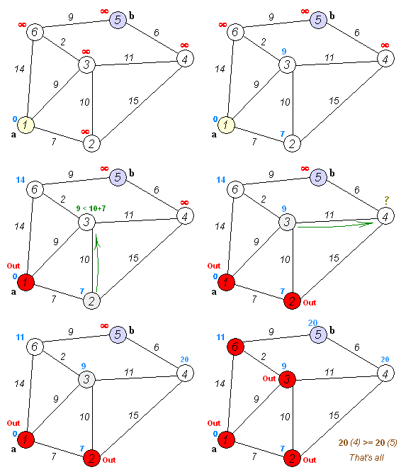
---- explain in more detail how it works

Network optimisation algorithm

• make sure links are not doubled (i.e. with a return trip), and if necessary reverse the start and end nodes.
• transform link set from arcs to segments (i.e. links with only two nodes).
• remove dead ends in the network (if a node has only one link)
• remove nodes from a junction-free section, and aggregate relevant data field (original link length and impedance)
• repeat removing dead-end and junction-free sections until no more nodes are removed.

Creating Origin-Destination matrices

Finding the path with the lowest impedance from A to B is relatively easy with Dijkstra's algorithm. However, for many applications, it is very useful to calculate this for a large set of origins and/or destinations.

Spatial interaction models

The following text comes from Nijkamp et al ()

Spatial Interaction Models are powerful tools and have been a source of intensive research in the past decades. Various spatial phenomena such as migration, passenger transport, international trade, shopping behavior and hospital admissions can all be described by models of this class. A very general and flexible Spatial Interaction Model was proposed by Alonso (1973, 1978). Alonso’s model contains equations for flows between regions, total outflow from a region, and total inflow to a region. The three components are connected by balancing factors. Alonso (1978) calls his model system a ‘A Theory of Movements’. It is also denoted as a ‘systemic model’, ‘Alonso’s General Theory of Movement’, ‘Three Component Model’ or ‘Extended Gravity Model’. There is not a standard name for the model. The term ‘Alonso-model’ is not suited for this model, as this mostly refers to Alonso’s (1964) model of urban land use. We will use here the term General Theory of Movement (GTM). This General Theory of Movement assumes a somewhat isolated position in the literature, and has not often been applied. This may be caused by lack of a clear interpretation, and by the difficulty to estimate the model econometrically. In this paper we will survey the GTM. We give a consistent formulation of Spatial Interaction Models and Alonso’s GTM, analyze the statistical properties of the GTM, and discuss its interpretation and estimation problems. In this way we hope to unveil the potential of this model.

Alonso’s General Theory of Movement stands in a tradition which started in the 19th century with the gravity model. Many spatial flow phenomena can be modelled as the product of the sizes of the origin and the destination, divided by a power function of distance. In the course of time various improvements of the model were proposed. A great step forward was made by Wilson (1967, 1970, 1974), who related Spatial Interaction Models to the entropy concept, and introduced a family of models: the unconstrained gravity model, the production constrained model, the attraction-constrained model and the doubly constrained model. Alonso’s GTM established a further improvement. Alonso (1973) developed his model as part of a large demographic model for the United States. The submodel for interregional migration is a Spatial Interaction Model, which offered a new specification of flows, inflows, outflows and their interrelationship. Alonso (1978) elaborated the model as a general framework for Spatial Interaction Models. Essentially the same model was independently developed by Bikker (1987, 1992) and Bikker and De Vos (1992) for international trade and hospital admissions.

In the first years after the presentation of the GTM by Alonso (1978), it stimulated a vivid discussion (Hua and Porell (1979), Anselin and Isard (1979), Hua (1980), Wilson (1980), Alonso (1980), Ledent (1980, 1981), Anselin (1982), Fotheringham and Dignan (1984), Tabuchi (1984)). This did not result, however, in a generally accepted view on the model. Standard works on Spatial Interaction Models as Batten and Boyce (1986), Fotheringham and O'Kelly (1989) and Nijkamp and Reggiani (1992) do mention Alonso’s model, but in most cases the model is not integrated in the treatment and no further pathways are explored. The situation has been sketched strikingly by Hua (1999):

“Many have been intrigued by this theory, and tried to clarify, to put it in operation, or to develop it further. But is seems frustration has prevailed and enthusiasm has been dampened somewhat now twenty years after the theory’s publication. This is not due to the exhaustion of possible development of the theory, but, to the contrary, to the non-conclusion of those studies on the theory. The mystery of the theory remains as it was and that has retarded the needed progress.”

We suggest that the confusion around the GTM can mainly be attributed to the role of two variables in the model, which are called ‘systemic variables’ or ‘balancing factors’. These variables are essential in the model, as they ensure the coherence and equilibrium in the system, but their interpretation is not clear. This has several consequences. In the first place, a clear view on the model is hampered by the fact that those mysterious variables occur in almost every equation. This means that those equations cannot be explained separately, but only in relation to the whole system of equations. Secondly, there is not an obvious single way to formulate the equations. Various representations of the model are possible, which can be derived from each other by substitutions or transformations (Hua (1999), Alonso (1978)). And thirdly, confusion arises around these variables in the process of estimation and prediction, as they are unobserved endogenous variables.

Several approaches can be thought of to interpret the GTM. The simplest is to see the model as an interpolation between the various members of Wilson’s Family of Spatial Interaction Models. It can be demonstrated that Alonso’s GTM contains the models of Wilson’s Family as special cases. The reverse is not true. The GTM is more flexible, as it enables interaction between flows and marginal totals (see Section 3). A change in transport costs on a single link, through new infrastructure, for example, will generally affect all flows and all marginal totals. Such a property is not found in Wilson’s family of models. The nature of the GTM can be clarified by studying the effect of changes in exogenous variables on the flows. This can be done for a change in a single value, or for overall changes. A more substantial approach is to give a direct interpretation of the balancing factors, by seeing them as (inverted) prices, shadowprices, or costs. Finally, the model could be derived from a more complex model, preferably an economic model, involving actors making choices based on prices.

The GTM is easy to compute. In most cases this can simply be done on a spreadsheet. Estimation of the parameters is, however, rather complicated. The balancing factors are unobserved, so they have to be estimated first. This can be achieved by estimating the allocation part of the model, and using the results to compute balancing factors. As these balancing factors are endogenous variables, the GTM is a simultaneous equation model, and application of Ordinary Least Squares (OLS) will produce biased and inconsistent estimates. Estimation by Instrumental Variables or Maximum Likelihood is then required.

The difference in notation and terminology used by various authors complicates research on the GTM. The model is studied by geographers, spatial economists and econometricians, and is very general; it can be applied to migration, international trade, transportation, hospital admissions, and other subjects. These various backgrounds lead to different choices of symbols, which are difficult to reconcile. Throughout this paper we will use a notation which is primarily based on the doubly constrained model of Wilson (1970, 1974), as it is also described in various survey works such as Wilson and Bennett (1985), Batten and Boyce (1986), De la Barra (1989), Fotheringham and O'Kelly (1989) and Nijkamp and Reggiani (1992). In this way we want to relate the GTM to the literature on Spatial Interaction Models. In the choice of additional symbols needed in the GTM we follow Alonso (1978) and Hua (1999).

Overview of usefule accessibility indicators

• travel time to reach x amount of people
• how many people can be reached within x minutes of travel
• average travel time to all populated cells within 120km Eucliean and within 4 hours
• potential accessibility to destination population with a distance decay function

Applications

• EU networks
• Public transport modelling

An important distinction needs to be made between:

• impedances in a Euclidean space (as the crow flies)
• impedances over a network

With the GeoDMS both types of impedances can be calculated, but usually, networks are used to calculate more realistic impedances. The GeoDMS contains network functions to build a network topology and use it in impedance functions to calculate impedances per origin point or in an origin/destination matrix (trip table).

Much attention has been given to making network calculations fast and efficient. This allows users to calculate impedances in large networks in a limited time.

applications

• Accessibility measures are calculated and used as driving factors for Land Use Modelling
• Origin Destination matrix (trip table) for many applications
• In our projects in the social domain, distances from houses to services are calculated. These distances are important suitability factors for housing for persons with mobility issues.

downloads

• PC4 travel time matrix for Nederland van Boven (in Dutch)