Repository navigation
Zoning and spatial units
Before any routing happens, a decision is made about what the origins and destinations are: individual addresses, postcode zones, municipalities, or grid cells. This decision introduces errors that no amount of routing precision can repair, and it is the most under-reported source of difference between accessibility studies.
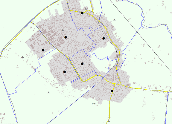
The geometric centroid of a zone (left) versus a population-weighted point derived from address data (right).
When a zone is represented by a single point, every dwelling in it is treated as if it were at that point. Two distinct problems follow:
- Intrazonal impedance is undefined. The distance from a zone to itself is zero by construction, which is wrong and matters most for exactly the short trips — walking to a shop, cycling to school — where accessibility differences are sharpest. Common fixes are a fraction of the zone's radius, or the mean distance between address pairs inside the zone.
- The representative point is a choice. A geometric centroid can fall in a lake, an industrial estate, or outside the zone entirely for a horseshoe-shaped municipality. A population-weighted point derived from address or building data is almost always better, and is what we use — see PC4 travel time matrix for Nederland van Boven for a worked example.
Aggregation error grows with zone size and with the heterogeneity inside the zone. It is largest in rural areas, where zones are big — which means it systematically distorts precisely the urban-versus-rural comparisons that accessibility studies are often commissioned to make.
Results depend on both the scale of the zoning and the way boundaries are drawn at that scale — the modifiable areal unit problem. Two zonings of the same country with the same number of zones can produce different rankings.
The practical response is not to solve it — it cannot be solved — but to bound it: compute the indicator at two or more spatial resolutions and report whether the conclusion holds.
| Unit | When appropriate | Cost |
|---|---|---|
| Addresses / buildings | Local studies, service-distance analysis, anything where short distances matter | Highest; millions of origins |
| Grid cells (100 m, 500 m) | National and continental studies, comparability across countries | Moderate; regular, no MAUP boundary effects but still scale effects |
| Postcode zones (PC4, PC6) | Where results must join to administrative or commercial data | Moderate; irregular sizes |
| Municipalities / regions | Policy reporting at that level only | Low; heavy aggregation error |
Note that origins and destinations need not use the same unit. A common and efficient pattern is fine-grained origins (where people live) against exact destination locations (where facilities are), which keeps precision where it matters without a full address-to-address matrix.
Destinations just outside the study area are invisible to the model, so locations near the boundary score artificially low. This is a data-extent problem, not a zoning one, but it shows up the same way on the map. Mitigate by extending the network and the destination set well beyond the study area — with a margin at least as large as the largest threshold or the effective range of the decay function. See Network data sources.

Concepts
Networks
- Network data sources
- OSM
- NWB
- GTFS
- Building a routable network
- Network optimisation algorithm
- Travel speeds per mode
Origins & destinations
Computation
- Shortest path and the Dijkstra algorithm
- Origin Destination matrix (trip table)
- Isochrones and catchment areas
- Public transport routing
Indicators
Applications
Network models
Reference