Gaussian_Process

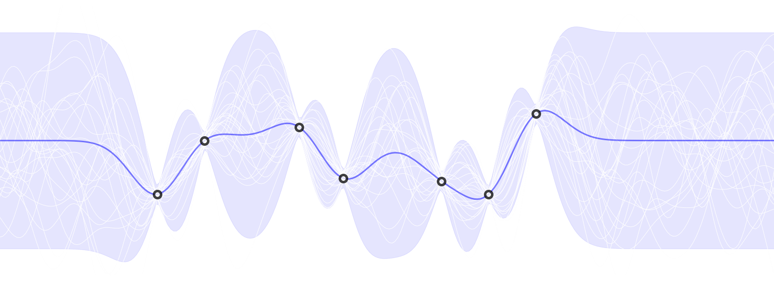
A gaussian process demo implemented by PyTorch, GPyTorch and NumPy.

A Gaussian process is a collection of random variables, any finite number of which have a joint Gaussian distribution.

Such a perspective comes from Rasmussen & Williams. Instead of the traditional linear regressions that produce numbers for prediction, a GP prediction is a distribution.

In standard linear regression, we have

$$ y_n = \mathbf{w}^{\top} \mathbf{x}_n \tag{1} $$

where $y_{n}∈\mathbb{R}$ is just a linear combination of the covariates $x_{n}∈\mathbb{R}^D$ for the $n$ th sample out of $N$ observations. Now, let us ignore the weights $\mathbf{w}$ and instead focus on the function $\mathbf{y}=\mathbf{f}(\mathbf{x})$. Furthermore, let’s talk about variables $\mathbf{f}$ instead of $\mathbf{y}$ to emphasize our interpretation of functions as random variables.

A jointly Gaussian random variable $\mathbf{f}$ is fully specified by a mean vector and covariance matrix. Thus, we can say that the function $\mathbf{f}(\mathbf{x})$ is fully specified by a mean function $\mathbf{f}(\mathbf{x})$ and covariance function $k(\mathbf{x_n},\mathbf{x_m})$ such that

$$ \begin{aligned} m(\mathbf{x}_n) &= \mathbb{E}[y_n] \\ &= \mathbb{E}[f(\mathbf{x}_n)] \\ \\ k(\mathbf{x}_n, \mathbf{x}_m) &= \mathbb{E}[(y_n - \mathbb{E}[y_n])(y_m - \mathbb{E}[y_m])^{\top}] \\ &= \mathbb{E}[(f(\mathbf{x_n}) - m(\mathbf{x_n}))(f(\mathbf{x_m}) - m(\mathbf{x_m}))^{\top}]. \end{aligned} \tag{2} $$

And here it comes the standard presentation of a Gaussian Process. Let's denote it as

$$ \mathbf{f} \sim \mathcal{GP}(m(\mathbf{x}), k(\mathbf{x}, \mathbf{x}^{\prime})). \tag{3} $$

As a well-known effective trick, the covariance function $k(\mathbf{x_n},\mathbf{x_m})$ can also be considered as the kernel functions which describe the similarity between data points. You've must heard about plenty of famous kernels in some specified fields of machine learning (i.e. SVM), like the RBF kernel or linear kernel. We use kernel functions to generate some specific priors, which like a disorganized functions distribution. We then force those functions to "agree" with our training data. So only the compliant priors will be left and finally yield a distribution of regression.

The purpose of the Gaussian Process kernel function is to measure the similarity or relationship between data points in the input space. It defines how the outputs (function values) at different input points are correlated with each other. By doing so, it encodes our prior beliefs about the smoothness or structure of the underlying function we are trying to model.

To implement a Gaussian Process (GP) model, we first set up our kernel function, let's say the Radial Basis Function (RBF) kernel. We then collect training data and compute the kernel (covariance) matrix for the data points. The matrix will have dimensions n x n, where n is the number of training data points. Each element $K_{ij}$ in the matrix represents the kernel function evaluated between data points $i$ and $j$. To account for noise in the observations, we add a small value (e.g., 1e-6) multiplied by the identity matrix to the kernel matrix. Then we can calculate the inverse and Cholesky decomposition. Finally, we make the prediction for new points and calculate the uncertainty.

The code gp_torch.py I present here is a more modern approach, simply using powerful PyTorch & GPyTorch. You can also check the detailed calculation in gp_calculate.py.