This work is the second project of the OpenCV Pytroch Course's. Its focus is image classification. Half of the score is based on implementation. The other half is based on model performance.
The dataset consists of 8,174 images in 13 Kenyan food type classes. Sample images of KenyanFood13 dataset and the number of images in each of the classes are shown below:
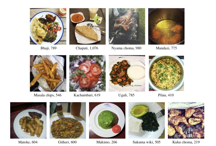
Figure 1: A sample image from each class of the KenyanFood13 dataset.
The data was split into public training set and private test set which is used for evaluation of submissions. The public set can be split into training and validation subsets.
To create a model that predicts a type of food represented on each image in the KenyanFood13 dataset's private test set. Pre-trained models may be used. The performance metric is accuracy. To receive any performance point, an accuracy of 70% must be achieved. To receive full points, an accuracy of 75% must be achieved.
Rather than create my own CNN architecture, I will explore transfer learning of models that have been trained on the ImageNet data set. Pedro Marcelino defines three strategies for fine-tuning pretrained models in Transfer learning from pre-trained models.
- Train the entire model
- Train some layers and leave others frozen
- Train only the classifer by freezing the convolutional base
Marcelino gives guidance as to which strategy to use based on one's dataset size and similarity (see Figure 2). Marcelino defines a small dataset as one with less than 1000 images per class. According to this definition, the KenyanFood13 dataset is small. However, it is unclear whether the application of data augmentation would reclassify the size of this dataset. Hence, this project will explore training the entire pretrained model as well as training some layers and leaving others frozen. Regarding dataset similarity, Marceline states:
... let common sense prevail. For example, if your task is to identify cats and dogs, ImageNet would be a similar dataset because it has images of cats and dogs. However, if your task is to identify cancer cells, ImageNet can’t be considered a similar dataset.
Fortunately, the ImageNet dataset contains 10 food classes: apple, banana, broccoli, burger, egg, french fries, hot dog, pizza, rice, and strawberry. Unfortunately, ImageNet's food images look significantly different from the images in Kenyan13Food dataset. Hence, the dataset similarity is moderate. Consequently, this project will also explore freezing the convolutional base and training only the classifier.
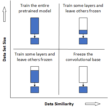
Figure 2: Decision map for fine-tuning pre-trained models.
According to the decision map, pre-trained models should be fine tuned by either freezing part or all of the convolutional base. This project will test the efficiency of this guidance.
Dishashree Gupta also defines strategies for fine-tuning pre-trained models in his blog post, Transfer learning and the art of using Pre-trained Models in Deep Learning. Gupta's strategies, while similar to Marcelino, have the following differences.
- Large datasets with low similarity should train models from scratch.
- Large datasets with high similarity should train the entire pre-trained model.
My primary objective is to fine-tune a pretrained model to achieve a minimum of 75% accuracy on the KenyanFood13 dataset. My secondary objective is to improve my proficiency with the Python computer programming language. Prior to this class, my Python expertise was almost non-existent. Consequently, I developed class hierachies that enable the rapid implementation of fine-tuning experiments on following pre-trained TorchVision and EfficientNet models using any of Marcelino or Gupta's strategies.
- ResNet-18
- ResNet-34
- ResNet-50
- ResNet-101
- ResNet-152
- ResNeXt-50-32x4d
- ResNeXt-101-32x8d
- Wide ResNet-50-2
- Wide ResNet-101-2
- VGG-11 with batch normalization
- VGG-13 with batch normalization
- VGG-16 with batch normalization
- VGG-19 with batch normalization
- DenseNet-121
- DenseNet-169
- DenseNet-201
- DenseNet-161
- EfficientNet-B0
- EfficientNet-B1
- EfficientNet-B2
- EfficientNet-B3
- EfficientNet-B4
- EfficientNet-B5
- EfficientNet-B6
- EfficientNet-B7
I used and modified the Trainer Pipeline module introduced in Week 6 - Best Practicing in Deep Learning > How to structure your Project for Scale. Modications to the trainer module include, but are not limited to, the following:
- additional configuration parameters,
- saving the model state only when the average loss on the validation set reaches a new low,
- prematurely stopping training when either the loss or accuracy does not significantly improve over a certain number of epochs, and
- extending the visualization base and TensorBoard classes to support the logging of images, figures, graphs, and PR curves.
Experiments are identified by three uppercase capital letters per the regular expression ([A-Z][A-Z][A-Z]). The first and second letters designate the experiment group and experiment set respectively. The last letter designates an individual experiment. Hence, all experiments that begin with "A" belong to Group A, while all experiments that begin with "AB" belong to Group A, Set B.
I implemented the following groups of experiments.
- Group A to explore the data and verify the training pipeline.
- Group B to explore the impact of learning rate on training pretrained EfficientNet models.
- Group C to explore the impact of EfficientNet model size and transfer learning approach on bias and variance.
- Group D to explore the impact of additional regularization and dataset imbalance approaches.
- Group E to explore the impact of a two-stage classifier.
- Group F to explore training the Project 1 model from scratch.
- Group G to explore and compare ResNet, ResNeXt, WideResnet, VGG, DenseNet, and EfficientNet models.
- Group H to explore model ensembles.
This first set of experiments logs contact sheets, 6 x 6 grids of images, of each food type to the visualizer with and without data augmentation.
The second set of experiments train only the classifier layer (fc) of the pre-trained Resnet18 model using a subset of the data without augmentation to check the training pipeline. In the first experiment, training will stop after 100 epochs. In the second experiment, training will stop after 100 epochs or when the smoothed accuracy (computed by expontential moving average with an alpha = 0.3) does not decrease by 2% within 10 epochs.
The third set of experiments varies the number of data loader worker threads to determine the optimal number for future experiments. These experiments stop after 11 epochs. The time between logging the first and eleventh epochs' test metrics divided by 10 will be used to evaluate data loading efficiency. Since the purpose to evaluate data loading, not the forward/back-propogation training cycle, a smaller model, ResNet18, was used. Furthermore, saving the model's state is disabled to eliminate its time contribution.
I used the data augmentation transforms I created for project 1. The data validation experiment revealed issues with these transforms. First, the color jitter transform dramatically changed the image's color. While this was not detrimental to classifying cats, dogs, and pandas; I suspect it may reduce accuracy on the KenyanFood13 dataset. Second, the amount of translation and scaling was too agressive.
To properly set the data augmentation transform parameters, I ran several experiments not shown in this notebook. These experiments disabled all but one type of augmentation in order to "tune" it. For example, to properly set the hue parameter of the color jitter transform, I disabled the horizontal/vertical flips, affine, and erase transforms. Furthermore, I set the color jitter's brightness, contrast, and saturation to the values that would produce the original image. I then found acceptable minimum and maximum values for the hue parameter. After conducting all of these data augmentation tuning experiments, I updated the configuration file and re-ran the data visualization experiment. I visualized the entire dataset to external files, but only logged the following 6 x 6 contact sheets to Tensorboard.
- ExpAAA - Original Images
- ExpAAA - "Tuned" Augmented Images
- ExpAAB - "Untuned" Augmented Images
The training pipeline check experiment performed as expected. The training and test loss decreased and the accuracy increased to approximtely 60%.
The results of the data loader experiments are shown below. For a small number of data loader threads, adding additional threads significantly increases the data loader's efficiency thereby allowing it to keep up with the GPU. However, past six or seven threads, the impact is minimal on a small model.
Table A1. The impact of the number of data loader worker threads on a training cycle.
| Experiment | Workers | Time/Epoch |
|---|---|---|
| ACA | 1 | 02:23 |
| ACB | 2 | 01:16 |
| ACC | 3 | 00:53 |
| ACD | 4 | 00:40 |
| ACE | 5 | 00:33 |
| ACF | 6 | 00:28 |
| ACG | 7 | 00:25 |
| ACH | 8 | 00:22 |
| ACI | 9 | 00:22 |
| ACJ | 10 | 00:22 |
| ACK | 11 | 00:21 |
| ACL | 12 | 00:21 |
| ACM | 13 | 00:20 |
| ACN | 14 | 00:19 |
| ACO | 15 | 00:18 |
| ACP | 16 | 00:18 |
The data augmentation looks reasonable. The training pipeline appears to work as expected. Since I am training models on a workstation with 8 hyper-threaded cores for a total of 16 CPUs and GPU acceleration, I dedicated 8 to 12 worker threads to the data loader. As the model complexity increases, the impact of fewer worker threads lessens because each worker has more time to load and transform images before the GPU requires the next batch.
The purpose of these experiments is to explore the impact of learning rate on training the following pretrained models.
- EfficientNet-B0 (Set A)
- EfficientNet-B2 (Set B)
- EfficientNet-B4 (Set C)
The entire network was trained, i.e., no layers were frozen. Each model was trained for 10 epochs with learning rates that varied between 1.00e-06 and 1.00e-02 with 4 learning rates per decade.
For each set of experiments, the following metrics were plotted as a function of learning rate in Figures B1, B2, and B3.
- Minimum test loss (min loss)
- Area under the test loss curve (auc loss)
- Test accuracy at the epoch of minimum test loss (accuracy)
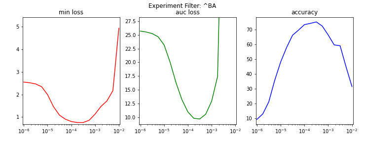
Figure B1. The impact of learning rate on the EfficientNet-B0 model.
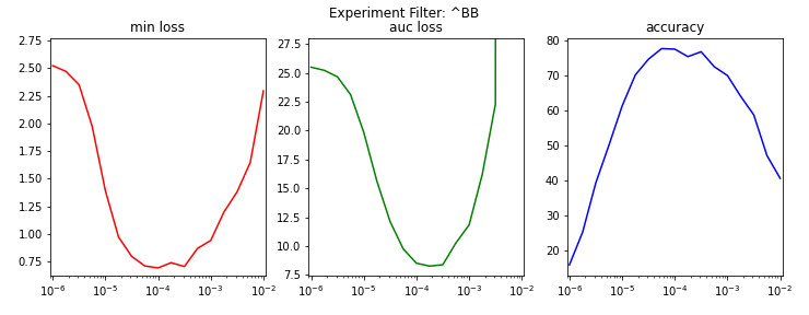
Figure B2. The impact of learning rate on the EfficientNet-B2 model.
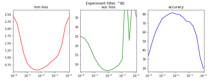
Figure B3. The impact of learning rate on the EfficientNet-B4 model.
Table B1 enumerates the aforementioned metrics for each set's experiment with the lowest test loss.
Table B1. The impact of learning rate on the EfficientNet models.
| Experiment | Learning Rate | Min Loss | AUC Loss | Accuracy |
|---|---|---|---|---|
| BAK_EfficientNetB0_PT5_LR3E-4 | 3.16e-04 | 0.76 | 9.69 | 75.22 |
| BBI_EfficientNetB2_PT5_LR1E-4 | 1.00e-04 | 0.69 | 8.51 | 77.63 |
| BCH_EfficientNetB4_PT5_LR6E-5 | 5.62e-05 | 0.57 | 6.80 | 81.88 |
The optimal learning rate appears to slightly decrease as the model complexity increases. Hence, a maximum learning rate of 1.00e-04 will be used in future EfficientNet experiments.
The purpose of these experiments is to explore the impact of EfficientNet model size on bias and variance. If the model is too small for the dataset, then the accuracy will suffer (high bias). However, if the model is too large for the dataset, then it will overfit the data (high variance). Hence, it is important to select the appropriately sized model for the KenyanFood13 dataset. The following pretrained EfficientNet models will be evaluated.
- EfficientNet-B3 (Set A)
- EfficientNet-B4 (Set B)
- EfficientNet-B5 (Set C)
- EfficientNet-B6 (Set D)
Each of the models under test will be trained using the following approaches to test the strategies given by Marcelino and Gupta.
- Only the classifier is trained (_PT0).
- The classifier and ~ 40% of convolutional base is trained (_PT2).
- The entire network is trained (_PT5).
The models were trained for 35 epochs. The learning rate started at 1.00E-04 and was multipied by the
The test accuracy at the epoch where the test loss is lowest is used to compare model bias. An overfitting metric was developed to compare model variance. The overfitting metric is computed as follows.
- The test loss is divided by the training loss at each epoch.
- The loss ratios are fitted to a line (polynomial of order 1).
- The overfitting metric is the slope of the best fit line.
The overfitting metric is zero is the test loss decreases at the same rate as the training loss. It increases as the test loss decreases at a slower rate than the training loss.
Tables C1, C2, and C3 enumerate the minimum test loss, test accuracy at the epoch with minimum test less, and overfitting metric for the three aforementioned transfer learning strategies. Figures C1, C2, C3 are loss plots from three sample runs. The first sample does not depict any overfitting. The second and third samples do show some overfitting.
Table C1: Analysis of runs where only the classifier is trained.
| Experiment | Test Loss | Accuracy | Overfitting Metric |
|---|---|---|---|
| CAA_EfficientNetB3_PT0 | 1.546 | 54.96 | -0.001 |
| CBA_EfficientNetB4_PT0 | 1.456 | 55.43 | -0.001 |
| CCA_EfficientNetB5_PT0 | 1.503 | 55.12 | -0.001 |
| CDA_EfficientNetB6_PT0 | 1.529 | 54.13 | -0.002 |
Table C2: Analysis of runs where classifier and ~ 40% of convolutional base is trained.
| Experiment | Test Loss | Accuracy | Overfitting Metric |
|---|---|---|---|
| CAB_EfficientNetB3_PT2 | 0.673 | 78.11 | 0.075 |
| CBB_EfficientNetB4_PT2 | 0.619 | 80.89 | 0.118 |
| CCB_EfficientNetB5_PT2 | 0.640 | 80.05 | 0.130 |
| CDB_EfficientNetB6_PT2 | 0.744 | 79.51 | 0.142 |
Table C3: Analysis of runs where the entire network is trained.
| Experiment | Test Loss | Accuracy | Overfitting Metric |
|---|---|---|---|
| CAC_EfficientNetB3_PT5 | 0.615 | 81.26 | 0.125 |
| CBC_EfficientNetB4_PT5 | 0.601 | 82.03 | 0.195 |
| CCC_EfficientNetB5_PT5 | 0.576 | 82.11 | 0.208 |
| CDC_EfficientNetB6_PT5 | 0.605 | 81.88 | 0.203 |
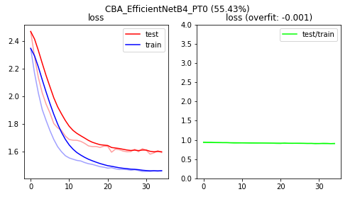
Figure C1: The loss plots of training only the classifier of a pretrained EfficientNet-B4 model.
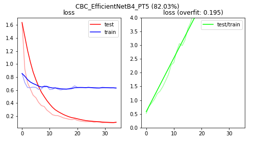
Figure C2: The loss plots of training the entire network of a pretrained EfficientNet-B4 model.
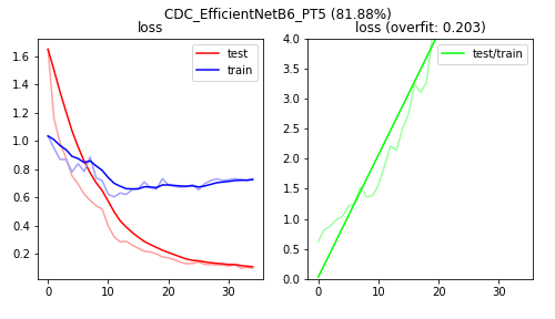
Figure C3: The loss plots of training the entire network of a pretrained EfficientNet-B6 model.
Training only the classifier of the EfficientNet models has a higher bias (lower accuracy) than training part of all of the convolutional base. Surprisingly, training the entire convolutional base yields slightly better accuracy than training the last 40% of the convolutional base. Regarding model complexity, the EfficientNet-B4 model seems appropriately sized.
This group of experiments explores the impact of increased regularization and dataset imbalance approaches. Because this project explores pretrained models, regularization options are limited. Gathering more data is not an option due to time constraints and lack of familarity with Kenyan food. Feasible regularization options include additional data augmentation and L2 / Ridge Regression.
This group has four sets.
- Set A explores increased data augmentation.
- Set B explores increased L2 regularization.
- Set C explores data imbalance approaches.
- Set D combines the "best" of the above.
Data augmentation was increased by adding shear, random color erasing, and Gaussian noise. Figures D1, D2, and D3 depict nine samples of chapati with no data augmentation, default data augmentation, and enhanced data augmentation respecitivity.
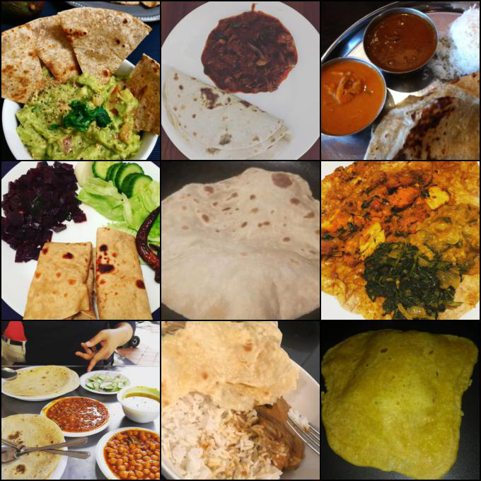
Figure D1: Nine samples of chapati with no data augmentation.

Figure D2: Nine samples of chapati with default data augmentation.
Figure D3: Nine samples of chapati with enhanced data augmentation.
Table D1 enumerates the results of the Group D experiments. Both the default and enhanced data augmentation reduced overfitting and increased the model's accuracy. The enhanced data augmentation reduced overfitting better than the default data augmentation at the expense of accuracy. L2 regularization likewise reduced overfitting at the expense of accuracy. Igoring dataset imbalance or using a weighted loss function slightly reduced accuracy. Combining a small increase in L2 regularization along with enhanced data augmentation slighly decreased accuracy.
Table D1: Analysis of Group D Experiments.
| Experiment | Test Loss | Accuracy | Overfitting Metric |
|---|---|---|---|
| DAA_EfficientNetB4_DA_NON | 0.722 | 77.37 | 1.238 |
| DAB_EfficientNetB4_DA_DEF | 0.551 | 82.87 | 0.076 |
| DAC_EfficientNetB4_DA_ENH | 0.584 | 80.50 | 0.056 |
| DBA_EfficientNetB4_WD_E-3 | 0.551 | 81.80 | 0.080 |
| DBB_EfficientNetB4_WD-E-2 | 0.622 | 79.74 | 0.042 |
| DBC_EfficientNetB4_WD_E-1 | 1.060 | 68.12 | 0.006 |
| DBD_EfficientNetB4_WD_E-0 | 2.005 | 36.09 | 0.004 |
| DCA_EfficientNetB4_DI_NON | 0.528 | 81.88 | 0.068 |
| DCB_EfficientNetB4_DI_WLF | 0.556 | 81.19 | 0.065 |
| DDA_EfficientNetB4_AS_DEF | 0.551 | 81.80 | 0.059 |
| DDB_EfficientNetB4_AS_ENH | 0.575 | 81.80 | 0.042 |
None of the experiments in this group improved the model's accuracy. Surprisingly, increasing regularization had a small detrimental impact on accuracy.
The confusion matrix from the most accurate models was re-ordered (in another notebook) using a greedy method so that the largest number of misclassifications were closest to the diagnoal. From this analysis, it was determined that a modest accuracy improvement was possible if models could more accurately classify images belonging to two or three classes rather than 13. The experiments in this group explore whether any of the theoretical improvements can be realized.
A two stage model with three second stages was implemented. The stage definitions are as follows. The numbers in backets are labels and the numbers after the colon are the number of samples in each class.
Stage1:
  [00] githeri: 479
  [01] mandazi: 620
  [02] masalachips: 438
  [03] matoke: 483
  [04] mukimo: 212
  [05] pilau: 329
  [06] group1: 1494
  [07] group2: 1451
  [08] group3: 1030

Stage2a:
  [00] bhaji: 632
  [01] chapati: 862

Stage2b:
  [00] kachumbari: 494
  [01] kukuchoma: 173
  [02] nyamachoma: 784

Stage2c:
  [00] sukumawiki: 402
  [01] ugali: 628
Table E1 enumerates the results of each stage as well as entire two-stage model. The first stage's accuracy was better than the best single stage model. Likewise, Stage2a accurately classified bhaji and chapati samples. Stage2b and Stage2c's accuracies were slighly lower than the best single stage model. Disappointingly, the two-stage model's accuracy was slightly lower than the best single stage model.
Table E1: The analysis of the two stage model.
| Experiment | Test Loss | Accuracy | Overfitting Metric |
|---|---|---|---|
| EAA_EfficientNetB4_Stage1 | 0.354 | 89.14 | 0.027 |
| EAB_EfficientNetB4_Stage2a | 0.170 | 94.00 | 0.019 |
| EAC_EfficientNetB4_Stage2b | 0.520 | 80.00 | 0.034 |
| EAD_EfficientNetB4_Stage2c | 0.543 | 80.56 | 0.051 |
| EAE_EfficientNetB4_TwoStage | 81.73 |
The confusion matrices of each stage are shown below in non-graphical form.
Two Stage - Accuracy: 81.72782874617737

[[ 95   7   0   2   0   4   1   2   2   1   5   1   6]
 [  8 157   0   1   0   0   0   1   0   0   1   1   3]
 [  1   2  91   0   0   0   1   0   0   0   0   0   1]
 [  2   1   2  68   3   2   0   0   0   9   4   2   6]
 [  0   0   0   1  20   0   1   1   0  12   0   0   0]
 [  1   0   0   0   1 121   0   0   0   0   0   0   1]
 [  3   0   0   1   1   0  82   0   0   0   0   0   1]
 [  6   2   1   0   0   1   1  79   1   1   1   1   3]
 [  0   0   1   0   0   1   2   1  34   0   0   1   2]
 [  2   5   1  11  10   2   1   0   0 117   4   0   4]
 [  0   0   0   0   0   0   0   1   0   0  63   2   0]
 [  0   3   4   3   0   1   0   3   0   1   1  43  21]
 [  0   1   0   5   0   0   0   3   0   3   0  15  99]]

[126 172  96  99  35 124  88  97  42 157  66  80 126]

1069 / 1308 = 0.8172782874617737

|Experiment|Test Loss|Accuracy|Overfitting Metric|
|:---|:---:|:---:|:---:|
|EAA_EfficientNetB4_Stage1|0.354|89.14|0.027|
|EAB_EfficientNetB4_Stage2a|0.170|94.00|0.019|
|EAC_EfficientNetB4_Stage2b|0.520|80.00|0.034|
|EAD_EfficientNetB4_Stage2c|0.543|80.56|0.051|

stage_results[0]

[[ 91   0   1   0   0   0   3   0   1]
 [  0 121   0   0   0   0   1   1   1]
 [  0   0  82   0   0   0   3   2   1]
 [  1   1   1  79   1   1   8   1   4]
 [  1   1   2   1  34   0   0   0   3]
 [  0   0   0   1   0  63   0   0   2]
 [  0   4   1   3   2   6 267   4  11]
 [  3   4   2   1   0   8  10 251  12]
 [  4   1   0   6   0   1   4  12 178]]

1166 / 1308 = 0.8914373088685015

stage_results[1]

[[ 95   7   0]
 [  8 157   0]
 [ 15  14   0]]

252 / 296 = 0.8513513513513513

stage_results[2]

[[ 68   3   9   0]
 [  1  20  12   0]
 [ 11  10 117   0]
 [ 12   2   6   0]]

205 / 271 = 0.7564575645756457

stage_results[3]

[[43 21  0]
 [15 99  0]
 [ 8 27  0]]

142 / 213 = 0.6666666666666666
The two-stage model's accuracy was slightly lower than the best single stage model's accuracy.
This group of experiments trains Project 1's model from scratch in order to compare its performance versus models developed by researchers who know a lot more than me.
After 160 epochs, the model achieved an accuracy of approximately 35%. When the experiment was terminated by Google Colabs, the test loss was still decreasing and the accuracy was increasing. It would be an interesting experiment to explore whether Cyclical Learning Rates for Training Neural Networks significantly decreases training time.
Transfer learning significantly decreases training time.
This group of experiments 1) trains the convolutional base and classifier of the following pretrained models and 2) compares their accuracies against the validation data.
- Set A
- ResNet-18
- ResNet-34
- ResNet-50
- ResNet-101
- ResNet-152
- Set B
- ResNeXt-50
- ResNeXt-101
- Set C
- WideResNet-50
- WideResNet-101
- Set D
- VGG11 w/ Batch Normalization
- VGG13 w/ Batch Normalization
- VGG16 w/ Batch Normalization
- VGG19 w/ Batch Normalization
- Set E
- DenseNet-121
- DenseNet-169
- DenseNet-201
- DenseNet-161
- Set F
- EfficientNet-B0
- EfficientNet-B1
- EfficientNet-B2
- EfficientNet-B3
- EfficientNet-B4
- EfficientNet-B5
- EfficientNet-B6
- EfficientNet-B7
The experiments were analyzed. Table G1 enumerates their results in descending order.
Table G1: Experiment results sorted by accuracy in descending order.
| Experiment | Test Loss | Accuracy | Overfitting Metric |
|---|---|---|---|
| GFF_EfficientNetB5_PT5 | 0.543 | 83.18 | 0.044 |
| GFE_EfficientNetB4_PT5 | 0.553 | 82.34 | 0.037 |
| GFG_EfficientNetB6_PT5 | 0.644 | 81.5 | 0.059 |
| GFH_EfficientNetB7_PT5 | 0.746 | 79.59 | 0.108 |
| GFD_EfficientNetB3_PT5 | 0.628 | 79.52 | 0.023 |
| GBA_ResNeXt50_PT5 | 0.691 | 78.74 | 0.102 |
| GED_DenseNet161_PT5 | 0.665 | 78.71 | 0.078 |
| GCA_WideResNet50_PT5 | 0.686 | 78.4 | 0.122 |
| GEC_DenseNet201_PT5 | 0.672 | 78.23 | 0.067 |
| GBB_ResNeXt101_PT5 | 0.731 | 77.51 | 0.475 |
| GAD_ResNet101_PT5 | 0.729 | 77.42 | 0.101 |
| GFC_EfficientNetB2_PT5 | 0.703 | 77.41 | 0.01 |
| GAC_ResNet50_PT5 | 0.728 | 77.02 | 0.053 |
| GEA_DenseNet121_PT5 | 0.717 | 76.88 | 0.019 |
| GCB_WideResNet101_PT5 | 0.744 | 76.56 | 0.196 |
| GDC_VGG16BN_PT5 | 0.787 | 76.53 | 0.048 |
| GAE_ResNet152_PT5 | 0.736 | 76.04 | 0.129 |
| GDD_VGG19BN_PT5 | 0.769 | 75.74 | 0.062 |
| GEB_DenseNet169_PT5 | 0.72 | 75.63 | 0.047 |
| GDB_VGG13BN_PT5 | 0.794 | 74.8 | 0.028 |
| GFB_EfficientNetB1_PT5 | 0.799 | 73.77 | 0.009 |
| GAB_ResNet34_PT5 | 0.784 | 73.57 | 0.033 |
| GDA_VGG11BN_PT5 | 0.814 | 73.15 | 0.023 |
| GAA_ResNet18_PT5 | 0.842 | 71.65 | 0.013 |
| GFA_EfficientNetB0_PT5 | 0.961 | 69.66 | 0.004 |
The EfficientNet-B5 model most accurately classified the KenyanFood13 validation data.
This set of experiment explores ensembles. As a prelimary test, all models resulting from the Group G experiments who accuracy was greater than or equal to 77% were assembled into an ensemble. The ensemble used three classification approaches.
- Combine model probabilities and use highest probability as prediction (AP).
- Select highest probablity as prediction (MP).
- Majority vote wins - ties broken by model with highest accuracy (V1).
- Majority vote wins - ties broken by model with highest probability (V2).
Next, the most accurate model, EfficientNet-B5, was trained on 15 different splits of the public data into training and validation data. Given these models have no common validation data, the models are passed to ensemble classifer without regard to their accuracy thereby rendering classification approach V1 meaningless. The test data will be classified by this ensemble using approaches AP, MP, and V2.
Predictions for the validation dataset were computed on ensembles comprised of two to 12 of the most accurate models of Group G via the three classification approaches. The accuracies of these predications are summarized in Table H1. The highest accuracy was 85.40%, which is 2.22% higher than the most accurate model. Unfortunately, the most accurate ensemble only achieved an accuracy on the test set of 82.746%, which is only 0.00729% higher than the most accurate model.
Table H1: The accuracy of the preliminary ensembles.
| Models | Pred_AP | Pred_MP | Pred_V1 | Pred_V2 |
|---|---|---|---|---|
| 02 | 83.56 | 84.02 | 83.18 | 84.02 |
| 03 | 83.87 | 83.87 | 83.64 | 84.02 |
| 04 | 84.17 | 83.87 | 84.48 | 84.17 |
| 05 | 84.94 | 84.10 | 85.09 | 85.02 |
| 06 | 84.56 | 84.02 | 85.17 | 85.17 |
| 07 | 84.79 | 84.02 | 85.40 | 85.09 |
| 08 | 84.86 | 83.94 | 84.79 | 84.56 |
| 09 | 84.94 | 84.40 | 84.48 | 84.71 |
| 10 | 84.63 | 84.40 | 84.33 | 83.94 |
| 11 | 84.48 | 84.40 | 84.33 | 84.40 |
| 12 | 83.94 | 84.17 | 83.79 | 83.64 |
My earlier testing determined the data loader's WeightedRandomSampler equally represented the KenyanFood13 dataset's classes during training. I decided to write test code to determine whether the images it selected were equally represented. Somewhat surprisingly, they were not. Hence, I wrote my own sampler that not only provided equal class representation, but also equal image representation during training. I used this sampler in the Group H, Set A experiments to train EfficientNet-B5 models. In addition, each of these experiments used a different random seed value. Hence, they each partitioned the public data into different training and validation sets. These training set were analyzed by counting how many experiments used eah image in the public dataset. Table H2 enumerates count statistics while Figure H1 depicts of count histogram. In hindsight, I should have manually partitioned the public data into training and validation sets to achieve more equal training exposure of the public images.
Table H2: The count statistics. On average each image in the public dataset is used by 11.998 experiments to train its model with a standard deviation of 1.584.
| Statistic | Value |
|---|---|
| minimum | 5 |
| maximum | 15 |
| median | 12 |
| mean | 11.998 |
| st dev | 1.584 |
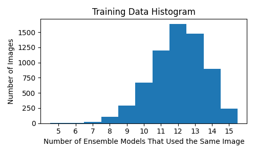
Figure H1: The number of public images used by N experiments during training.
Each experiment was analyzed and the results are enumerated in Table H3. The minimum, maximum, and average accuracies are 81.80%, 84.02%, and 82.84% respectively. Figure H2, H3, and H4 are the confusion matrices on the least accurate prediction, most accurate prediction, and an average prediction respectively. Note: Predictions were made of different validation datasets.
Table H3: The results of Group H, Set A experiments.
| Experiment | Test Loss | Accuracy | Overfitting Metric |
|---|---|---|---|
| HAA_EfficientNetB5_0042 | 0.584 | 82.80 | 0.089 |
| HAB_EfficientNetB5_5174 | 0.563 | 83.49 | 0.081 |
| HAC_EfficientNetB5_2123 | 0.621 | 82.57 | 0.093 |
| HAD_EfficientNetB5_6993 | 0.548 | 83.94 | 0.086 |
| HAE_EfficientNetB5_8133 | 0.579 | 82.65 | 0.104 |
| HAF_EfficientNetB5_0438 | 0.587 | 81.80 | 0.101 |
| HAG_EfficientNetB5_3708 | 0.571 | 83.41 | 0.096 |
| HAH_EfficientNetB5_0888 | 0.597 | 82.57 | 0.104 |
| HAI_EfficientNetB5_2984 | 0.598 | 82.65 | 0.103 |
| HAJ_EfficientNetB5_0565 | 0.557 | 82.87 | 0.098 |
| HAK_EfficientNetB5_6816 | 0.586 | 82.95 | 0.098 |
| HAL_EfficientNetB5_2956 | 0.591 | 81.80 | 0.102 |
| HAM_EfficientNetB5_1713 | 0.569 | 82.49 | 0.099 |
| HAN_EfficientNetB5_2570 | 0.571 | 84.02 | 0.101 |
| HAO_EfficientNetB5_1541 | 0.588 | 82.57 | 0.115 |
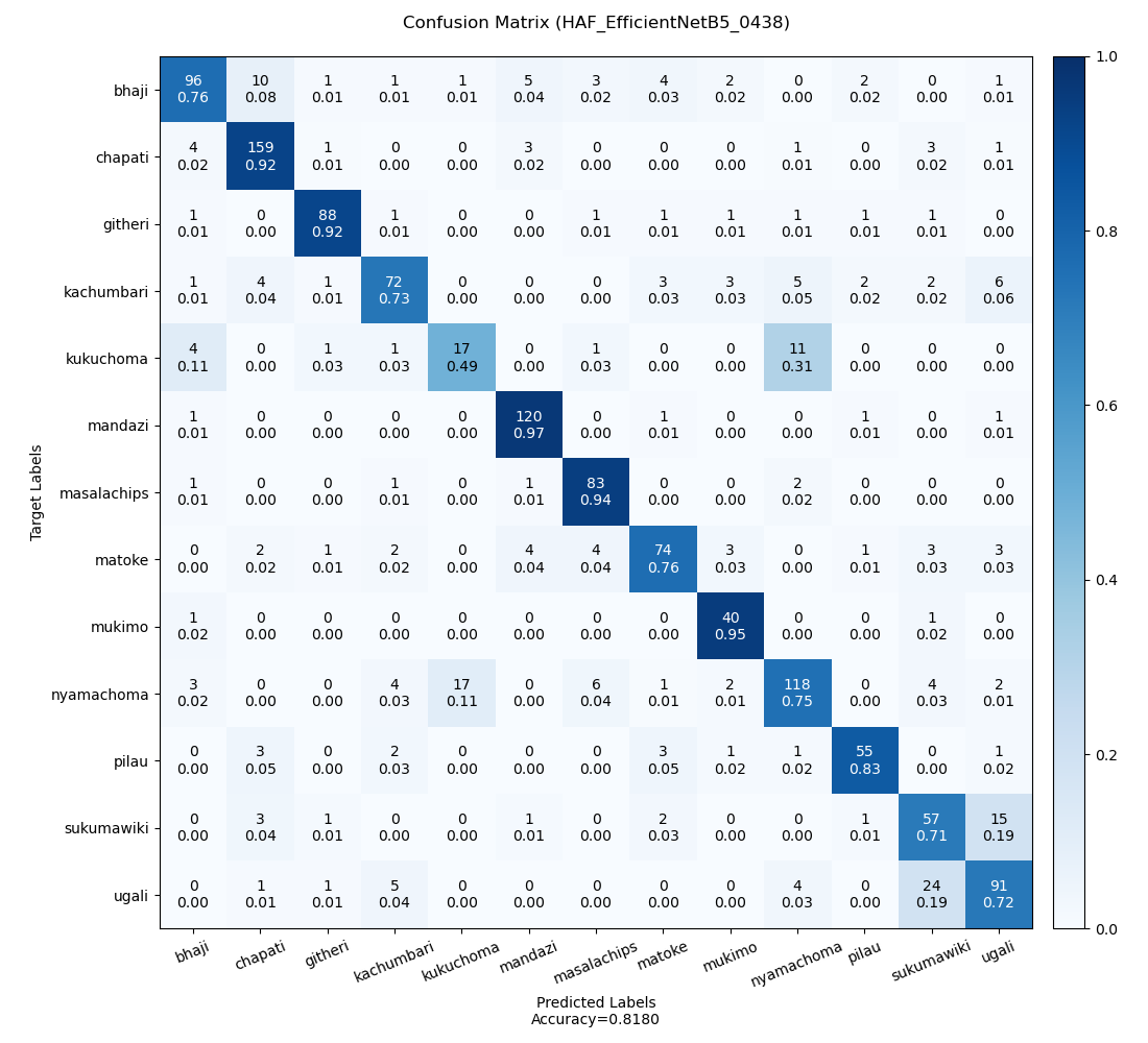
Figure H2: The confusion matrix for the least accurate prediction.

Figure H3: The confusion matrix for the most accurate prediction.
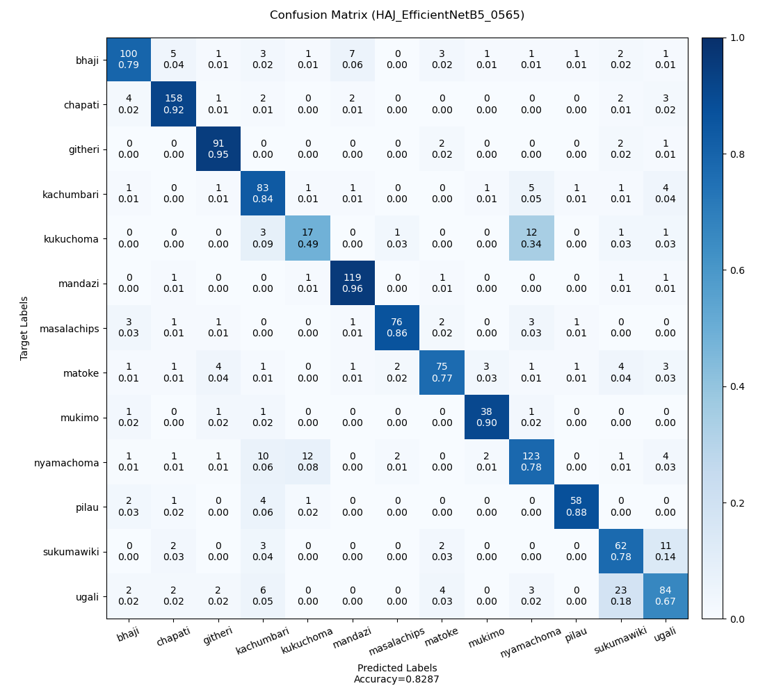
Figure H4: The confusion matrix for an average prediction.
Figure H5 visualizes the voting approaches. The x-axis are the indices of the test images. The y-axis is the highest number of models that predicted the same class. For the majority of test images, all models in the ensemble predicted the same class. All images had at least five models predict the same class.
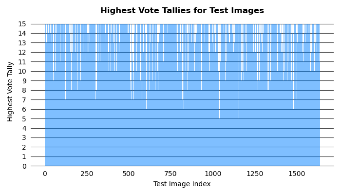
Figure H5: The highest vote tallies for all test images.
Predictions of the private data were made using the classification approaches AP, MP, and V2. They scored 82.867%,83.110%, and 82.867% respectively on Kaggle's Public Leaderboard.
The non-ensemble experiment with the best accuracy is GFF_EfficientNetB5_PT5. This experiment fine tuned the entire convolutional base and classifier of a pretrained EfficientNet-B5 model using the default data augmentation, my custom data loader sampler, and a very small L2 regularization. Its accuracy in classifying the samples in the validation set is 83.18%. Its accuracy on the test data is 82.017% according to the public Kaggle leaderboard. Its confusion matrix is depicted in Figure 3.
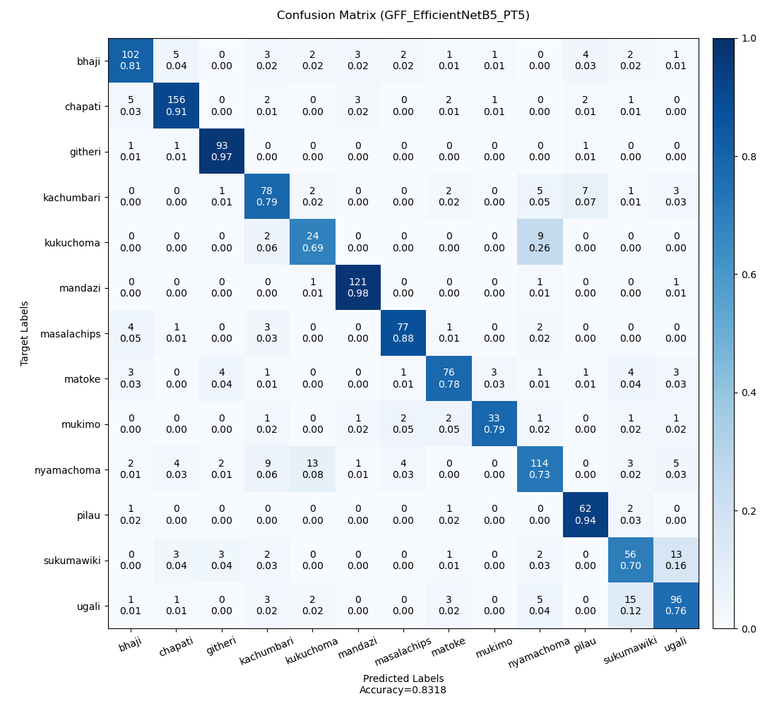
Figure 3: The confusion matrix of the most accurate model.
My most accurate prediction on Kaggle's Public Leadership is the FinalEnsemble, most probable predictions (Preds_MP). Its accuracy on the test data is 83.110% according to the public Kaggle leaderboard.
The following areas warrant attention.
- Investigate why increasing the regularization not only reduced overfitting, but also reduced the model's accuracy.
- Investigate whether the accuracies of the second stages of the two-stage model could be increased, thereby increasing the overall accuracy of the two-stage model.
In general, the models confused the following classes.
- kukuchoma and nyamachoma
- sukumawiki and ugali
Future exploration should focus on distinguishing between these classes.