EDA-and-Machine-Learning

Overview

This notebook models a given data set using the classification technique. It also uses various preprocessing & Exploratory data analysis steps.

Requirements

Libraries used and their versions:

1. Numpy==1.19.2
2. Pandas==1.1.3
3. Matplotlib==3.3.2
4. Seaborn==0.11.0
5. Statsmodels==0.12.0
6. Scikit-Learn==0.23.2

---

The notebook contains 5 major sections:

1. Data preprocessing and EDA
2. Feature Engineering
3. Model building
4. Final model performance using best hyperparameters
5. Prediction of test data

Data preprocessing and EDA

In this step, I have first eliminated the first column with serial numbers, after reading the training data. Then used df.shape to check the dimensions. The df.describe() showed the range for all features are different, for example max value of X1 is 4.34 but for X57 its more than 10K. Hence, scaling will be used later. There were no null values present and all of the features were numerical, hence no encoding was required. A class imbalance was found using df['Y'].value_counts() method.

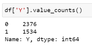
There are many methods to tackle class imbalance like collecting more data, duplication of data for which labels are less or deleting data for which labels are more etc. Here. we will using weight assigning technique, wherein we will assign more weights to label 1 and less weights to label 0 while training, using the formula:

weight = total_samples / (n_classes * class_samples)

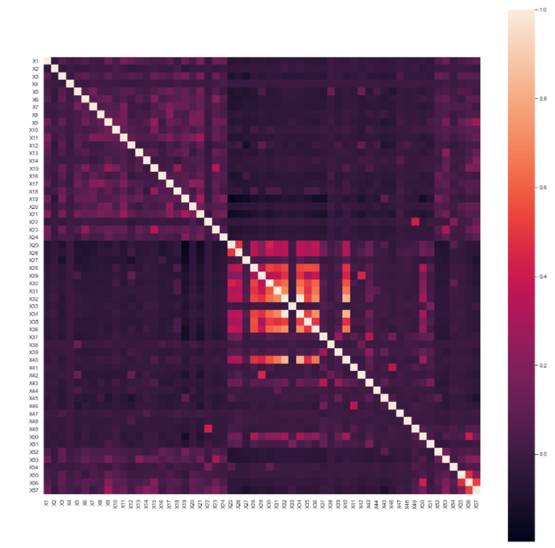
On checking linear correlation between different features, it was found that features X32 and X34 were highly correlated with each other. Also, few features like in the middle region also seem to be correlated with each other to certain extent, as shown below.

I tried removing outliers using IQR technique, but it did not work for the data set, as masking lead to many missing values.

Feature Engineering

In this first step I did was calculate Variance Inflation Factor of all the features. From this, I found that features X32 and X34 had a very high VIF, which strengthens our previous claim in EDA step. Hence, we will be removing one of them while and checking the VIF again and repeat till there are no features with VIF > 5. Below image shows the two said features with a high VIF:

I divided the data in train and validation part, where I reserved 20 % of total training data for validation. I also scaled the data, as mentioned in the EDA step. After that we use ANOVA using f_classif function to get p-values. Here, X38 & X12 have p-values > 0.05, so that should be removed.

Then I used SelectKBest() function to get first 35 most significant features, to be used for modeling (by trial and error). Those feature were:

['X1', 'X3', 'X5', 'X6', 'X7', 'X8', 'X9', 'X10', 'X11', 'X15', 'X16', 'X17', 'X18', 'X19', 'X20', 'X21', 'X23', 'X24', 'X25', 'X26', 'X27', 'X28', 'X29', 'X30', 'X35', 'X36', 'X37', 'X42', 'X43', 'X45', 'X46', 'X52', 'X53', 'X56', 'X57']

Model Building

For this I considered 2 methods:

• Logistic Regression
• KNN

Model performance analysis

For Logistic regression, we considered 4 iterations with different features. We also considered weights as discussed above in the EDA step.

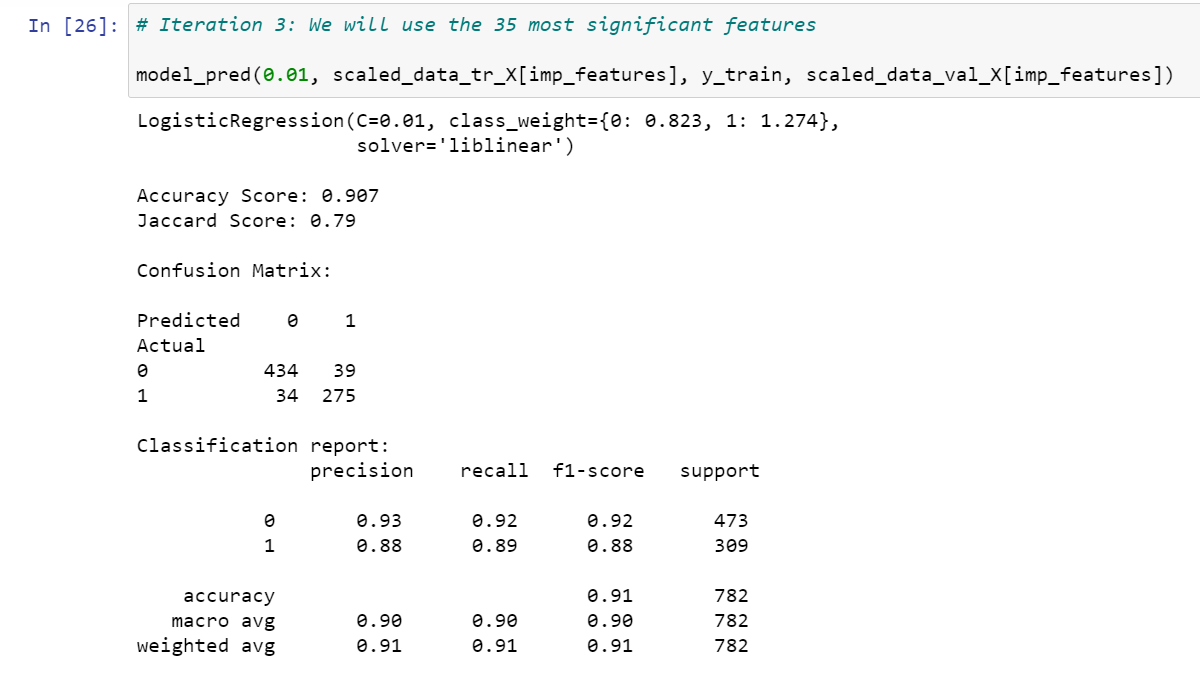
In first iteration, I considered all features including those with high VIF and p-value and in Second iteration, dropped X38 and X12, as they had high p-values, for comparison. In third, I used 35 most significant features and got validation f1-score of 0.91.

Before doing iteration 4, I dropped X38, X12 due to high p_value & also X32 due to high VIF and recheck VIF. It was found none of the entries now have VIF > 5. We preoceed to model with this data and found validation f1-score of 0.90, less than iteration 3.

We will neglect first two, as they had insignificant and high VIF features and take model of Iteration 3 for further consideration, as it had better f1-score and no high VIF and p-value features and it also uses lesser number of features i.e. 35.

Below image shows results for iteration 3.

For KNN, it was found f1-score was 0.90 i.e lesser than Logisitc regression, hence we will stick with the Logistic model of iteration 3.

GridSearchCV

I used GridSearchCV to get the best hyper-parameters for the model obtained from Iteration 3. Follwing are the best hyper-parameters:

The training accuracy score is 0.924 as seen above.

Final model performance using best hyperparameters

Finally we will check performance of the above model:

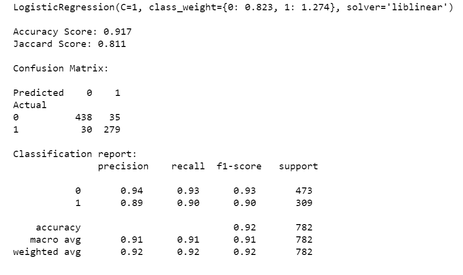
It can be seen the Final Validation f1-score is now 0.92, which is better than that of previous 0.91.

Prediction of test data

For prediction, I first read the csv file, did some checks to see if it has any null values. Then I scaled the test data, selected those 35 features that I considered while training and predicted the outcome with our final model. Then I appended the prediction with original test file and saved it as test_set_prediction.csv.