NOTE: This repository has been superceeded by the Rwclust package

weighted_graph_clustering

This repository contains an implementation of the weighted graph clustering algorithm based on random walks developed by Harel and Koren (http://www.wisdom.weizmann.ac.il/~harel/papers/Clustering_FSTTCS.pdf).

The procedure consists of two parts. The first part is an interative "edge sharpening" procedure that increases the weights of edges of non-cut edges and shrinks the weights of cut edges. This can serve as a preprocessing step for hierarchical clustering. This is implemented in the sharpenEdgeWeights function.

The next step is clustering, implemented in the findClusters function. There are three clustering methods supported. The first method deletes edges with edge weights below a certain cutoff threshold. The resulting connected components are the clusters. Single linkage clustering is also supported. Another hierarchical clustering method developed by the authors measures the distance between clusters as the normalized sum of edge weights between them. This method is also supported. See paper for details.

Usage

We will demonstrate how to use these methods using the two examples found in the original paper. The functions require the network and matrixcalc packages. Check out the example code in the /examples folder along with example data.

Edge-deletion method

First we load the data, which consists of a 3-column dataframe where the first two columns contain the edgelist and the third contains the weights.

test_graph1 <- read.csv("./examples/test_graph1.csv", stringsAsFactors = FALSE)

Next we create a weighted graph object using network. It important that the "weight" attribute be set and named.

G1 <- network(test_graph1, matrix.type = "edgelist", directed = FALSE)
set.edge.attribute(G1, "weight", test_graph1$weight)

Lets view the graph.

plot(G1)

Next we apply the edge sharpening procedure. The sharpenEdgeWeights takes four parameters, the weighted network object, the length of the longest walk k, the number of iteration steps the algorithm should take and whether or not to plot the histogram of edge weights. The edge weight histogram is used to select cutoff values for edge-deletion method. The sharpenEdgeWeights function returns a named list containing a network object with the new weights, the parameters "k" and "steps", the weighted adjacency matrix and the range of the edge weights. The outout is then passed on to the findClusters function.

results <- sharpenEdgeWeights(G1, k = 3, steps = 4, plot = TRUE)

Next we use the findClusters method using the cutoff of 0.97 used by the authors for this example.

new_G1 <- findClusters(results, method = "deletion", cutoff = 0.97, plot = TRUE)

When the findClusters uses the "deletion" method, a named list is returned containing a new network object and a vector of cluster assignments.

plot(new_G1$graph)

Hierarchical Clustering

# load data
test_graph2 <- read.csv("./examples/test_graph2.csv", stringsAsFactors = FALSE)
# create weighted graph
G2 <- network(test_graph2, matrix.type = "edgelist", directed = FALSE)
set.edge.attribute(G2, "weight", test_graph2$weight)
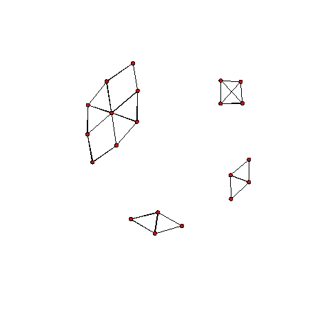
plot(G2)

# sharpen edge weights
results <- sharpenEdgeWeights(G2, plot = FALSE)

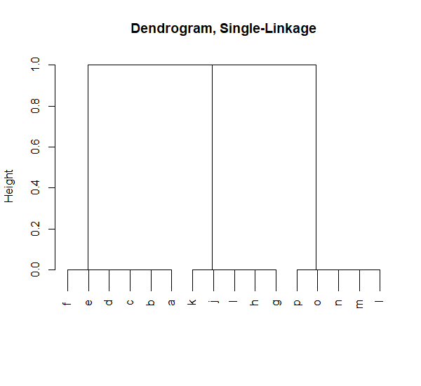
We can see there are three obvious clusters. We apply the two hierarchical clustering methods to find them. First we apply single linkage clustering on the graph.

results_1 <- findClusters(results, method = "single", plot = TRUE)

Next lets apply the normalized edge weight sum method.

results_2 <- findClusters(results, method = "normalized", plot = TRUE)