52 Must-Know GANs Interview Questions in 2026

You can also find all 52 answers here 👉 Devinterview.io - GANs

1. What are Generative Adversarial Networks (GANs)?

Generative Adversarial Networks (GANs) are a pair of neural networks which work simultaneously. One generates data, while the other critiques the generated data. This feedback loop leads to the continual improvement of both networks.

Core Components

• Generator (G): Produces synthetic data in an effort to closely mimic real data.
• Discriminator (D): Assesses the data produced by the generator, attempting to discern between real and generated data.

Two-Player Game

The networks engage in a minimax game where:

• The generator tries to produce data that's indistinguishable from real data to "fool" the discriminator.
• The discriminator aims to correctly distinguish between real and generated data to send feedback to the generator.

This training approach encourages both networks to improve continually, trying to outperform each other.

Mathematical Representation

In a GAN, training seeks to find the Nash equilibrium of a two-player game. This is formulated as:

$$ \min_{G} \max_{D} V(D, G) = \mathbb{E}_x[\log D(x)] + \mathbb{E}_z[\log(1 - D(G(z)))] $$

Where:

• $G$ tries to minimize this objective when combined with the maximization objective of $D$.
• $V(D, G)$ represents the value function, i.e., how good the generator is at "fooling" the discriminator.

Training Mechanism

1. Batch Selection: The training begins with a random set of real data samples $x_i$ and an equal-sized group of noise samples $z_i$.

2. Generator Output: The generator fabricates samples $G(z_i)$.

3. Discriminator Evaluation: Both real and fake samples $x_i$ and $G(z_i)$ are input into the discriminator, which provides discernment scores.

4. Loss Calculation: The loss for each network is calculated, with the aim of guiding the networks in the right direction.

5. Parameter Update: The parameters of both networks are updated based on the calculated losses.

6. Alternate Training: This process is iterated, with a typical alternation rate of one update for each network after multiple updates of the other.

Loss Functions

• Generator Loss: $-\log(D(G(z)))$. This loss function encourages the generator to produce outputs that would be assessed close to "real" (achieve a high score) by the discriminator.
• Discriminator Loss: It combines two losses from different sources:
  • For real data: $-\log(D(x))$ to maximize the score it assigns to real samples.
  • For generated data: $-\log(1 - D(G(z)))$ to minimize the score for generated samples.

GAN Business Use-Cases

• Data Augmentation: GANs can synthesize additional training data, especially when the available dataset is limited.
• Superior Synthetic Data: They are adept at producing high-quality, realistic synthetic data, essential for various applications, particularly in computer vision.
• Anomaly Detection: GANs specialized in anomaly detection can help identify irregularities in datasets, like fraudulent transactions.

Practical Challenges

• Training Instability: The "minimax" training equilibrium can be difficult to achieve, sometimes leading to the "mode collapse" problem where the generator produces only a limited variation of outputs.
• Hyperparameter Sensitivity: GANs can be extremely sensitive to various hyperparameters.
• Evaluation Metrics: Measuring how "good" a GAN is at generating data can be challenging.

GANs & Adversarial Learning

The framework of GANs extends to various contexts, leading to the development of different adversarial learning methods:

• Conditional GANs: They integrate additional information (like class labels) during generation.
• CycleGANs: These are equipped for unpaired image-to-image translation.
• Wasserstein GANs: They use the Wasserstein distance for the loss function instead of the KL divergence, offering a more stable training mechanism.
• BigGANs: Specially designed to generate high-resolution, high-quality images.

The adaptability and versatility of GANs are evident in their efficacy across diverse domains, including image generation, text-to-image synthesis, and video generation.

2. Could you describe the architecture of a basic GAN?

The basic architecture of a Generative Adversarial Network (GAN) involves two neural networks, the generator and the discriminator, that play a minimax game against each other.

Here is how the two networks are structured:

The Generator

The job of the Generator is to create data that is similar to the genuine data. It does this by learning the underlying structure and distribution of the training data, then generates new samples accordingly.

Neural Network Architecture

• Often uses a deconvolutional network (also known as a transposed convolutional neural network) to up-sample the data from a low-resolution, high-dimensionality noise variable (usually Gaussian) to the original data distribution

The Discriminator

The Discriminator is a classic binary classifier that aims to distinguish between real data from the training set and fake data produced by the Generator.

Neural Network Architecture

• Typically designed as a standard convolutional neural network (CNN) to handle high-dimensional grid data such as images
• Employs a binary classification head that predicts with high probability whether its input comes from the real data distribution or the fake data distribution, as generated by the Generator.

Network Training

The two networks engage in adversarial training, where the Generator takes in feedback from the Discriminator to learn and generate better samples, while the Discriminator updates to improve its ability to distinguish between real and fake samples.

The learning is achieved through minibatch stochastic gradient descent. The overall training algorithm is guided by the Adversarial Loss, which is a combination of the Discriminator's loss (typically a Binary Cross-Entropy Loss, BCELoss) and the Generator's loss.

Root Mean Squared Error Calculation

In the context of GANs, the discriminator's loss, often measured as BCELoss, can be used to downstream the loss through the backpropagation algorithm to update the generator's weights.

The Loss function is calculated as:

$$ \text{RMSE} = \sqrt{\frac{1}{N} \sum_{i=1}^{N} \left(y_{\text{true}} - y_{\text{pred}}\right)^2} $$

Here, $N$ is the number of samples, $y_{\text{true}}$ represents the true label, and $y_{\text{pred}}$ is the predicted probability by the discriminator that a sample belongs to the real data distribution (associated with the label 1).

The generated samples are then evaluated using the trained discriminator. If they are classified as real with high probability, the RMS error will be less, implying a higher likelihood of the generated sample being close to the real data distribution.

3. Explain the roles of the generator and discriminator in a GAN.

In a traditional Generative Adversarial Network (GAN), the generator and the discriminator play opposing roles:

1. Generator: Creates synthetic data to mimic the real data.
2. Discriminator: Learns to distinguish between real and fake data.

The goal is to optimize these two in tandem until the generator creates increasingly convincing outputs. This duel is often described as a "cat and mouse game" or "counterfeiter and detective situation."

GAN Training Algorithm

1. Initial Training: The data generator creates a batch of fake data, and the discriminator is trained to differentiate between real and fake samples. The generator's performance is then evaluated through the discriminator's feedback.

2. Updates: Each model is updated in alternating steps, one at a time:

   • The generator receives feedback from the discriminator.
   • The discriminator is updated based on a mix of real and fake data.

Code Example: Core GAN Training Steps

Here is the Python code:

for epoch in range(num_epochs):
    for batch_index in range(num_batches):
      
        # Update the discriminator
        real_data = get_real_data()
        fake_data = generator.generate_fake_data()
        d_loss = discriminator.train(real_data, fake_data)
      
        # Update the generator
        generated_data = generator.generate_fake_data()
        g_loss = discriminator.get_loss(generated_data)
        generator.train(g_loss)

• The discriminator is trained to classify real and fake data, aiming to maximize its accuracy. It receives mixed batches of real and fake data for training.

• The generator takes the feedback from the discriminator to improve its generated data quality, aiming to minimize the discriminator's ability to classify the output as "fake."

4. How do GANs handle the generation of new, unseen data?

Generative Adversarial Networks (GANs) have revolutionized unsupervised learning by pairing a generator and a discriminator in a competitive framework.

Data Generation Process in GANs

• Generator Network: Learns to synthesize data samples that are indistinguishable from real data.
• Discriminator Network: Trained to distinguish between real and generated data.

The generator and discriminator are constantly competing, leading to increasingly sophisticated models. The generator aims to trick the discriminator, while the discriminator tries to sharpen its ability to discern genuine data from synthetic data.

Challenges in Data Generation

1. Overfitting and Mode Collapse: The GAN can get stuck by producing limited types of data, leading to mode collapse as it fails to explore the complete data distribution.

2. Stochastic Data Output: Even an optimally trained GAN can yield some variability in the data it generates.

3. Sample Quality Control: The quality of generated data evolves over training time and isn't assured consistently.

Strategies for Enhanced Data Generation

To overcome these challenges and achieve robust, high-quality data generation, several techniques have been developed, such as:

• Regularization Methods: Introducing mechanisms like "Random Noise Injection" and "Feature Matching" can enhance the stability of GAN training and reduce mode collapse.

• Ensemble Approaches: Using multiple GANs in parallel and then averaging their outputs can lead to improved data generation.

• Post-Processing Techniques: After generation, passing the data through an additional processing step can boost its quality.

Evaluating Generated Data Quality

The quality of data generated by a GAN, compared to original data, often involves subjective and qualitative assessments. While quantitative metrics like Inception Score or Frechet Inception Distance are sometimes used, they have their limitations and may not always align with human judgment.

Ensuring consistent, high-quality data generated by GANs remains an active area of research.

5. What loss functions are commonly used in GANs and why?

The commonly used loss functions in Generative Adversarial Networks (GANs) are Binary Cross Entropy, Wasserstein Loss, and Hinge Loss.

Each loss function optimizes the GANs in unique ways to achieve certain properties, hence making them suitable for different types of problems.

Binary Cross Entropy

The Binary Cross Entropy (BCE) is the most common loss used in GANs, especially in the original GAN architecture proposed by Goodfellow et al.

The BCE is calculated between the real/fake labels (1s/0s) and the discriminator's predictions. The aim is to minimize this BCE loss, which forces the discriminator to accurately differentiate between real and generated samples.

For the generator, the BCE loss is calculated with an inverted label (real becomes fake, and vice versa). So, the generator tries to minimize the discrimination by the discriminator.

In Python using Pytorch, the BCE loss implementation could look like this:

# the BCE loss function
criterion = nn.BCELoss()

# Discriminator loss for real images
D_real_loss = criterion(D_real, torch.ones_like(D_real))

# Discriminator loss for fake images
D_fake_loss = criterion(D_fake, torch.zeros_like(D_fake))

# Total discriminator loss
D_loss = D_real_loss + D_fake_loss

# Generator loss
G_loss = criterion(D_fake, torch.ones_like(D_fake))

Wasserstein Loss

The Wasserstein Loss, used in Wasserstein GAN (WGAN), provides a more stable convergence and mitigates the problems of mode collapse (when GANs produce limited varieties of samples).

Here, the discriminator (critic in WGAN terminology) is trained to output a scalar score instead of a probability. In turn, the generator is trained to generate data that gets a higher score from the critic.

Here's a simple implementation on how you can use Wasserstein loss:

# Discriminator loss
D_loss = -(torch.mean(D_real) - torch.mean(D_fake))

# Generator loss
G_loss = -torch.mean(D_fake)

Hinge Loss

The Hinge Loss is used in the Spectral Normalization GAN (SNGAN). It encourages the margin between the positive and negative samples, helping the GAN to attain better performance.

# Discriminator loss
D_loss = -torch.mean(torch.min(D_real - 1, torch.zeros_like(D_real))) - torch.mean(torch.min(-D_fake - 1, torch.zeros_like(D_fake)))

# Generator loss
G_loss = -torch.mean(D_fake)

6. How is the training process different for the generator and discriminator?

During training of GANs (Generative Adversarial Networks), the generator and discriminator networks undergo unique optimization processes. Let's delve into the distinct training mechanisms for each network.

Discriminator's Training

The primary task of the discriminator is to distinguish between real and generated data.

1. Loss Calculation:

   • It starts with a loss evaluation based on its current performance. The loss is typically a binary cross-entropy, measuring the divergence between predicted and actual classes.

2. Backpropagation and Gradient Descent:

   • Backpropagation computes the gradients with respect to the loss.
   • The discriminator then alters its parameters to minimize this loss, typically through gradient descent.

Code example: Discriminator Training

Here is the Python code:

import torch
import torch.nn as nn
import torch.optim as optim

# Assuming discriminator_loss and discriminator_model are defined
discriminator_optimizer = optim.SGD(discriminator_model.parameters(), lr=0.001)

# Forward pass and loss calculation
real_data = torch.rand(32, 100)  # Example real data
predictions = discriminator_model(real_data)
loss = discriminator_loss(predictions, torch.ones_like(predictions))

# Backpropagation and parameter update
discriminator_optimizer.zero_grad()
loss.backward()
discriminator_optimizer.step()

Generator's Training

The generator aims to produce data that is indistinguishable from real data.

1. Loss Calculation:

   • Its loss is computed based on how well the generated data is classified as real by the discriminator. In this setup, the loss is the same binary cross-entropy loss, but the target label is flipped.

2. Backpropagation Through the Discriminator:

   • Surprisingly, the gradient doesn't stop at the discriminator. Backpropagation starts with the discriminator's output and then goes through the generator to compute the gradients. This is made possible by the detach method in PyTorch or using the non-suite tf.stop_gradient method in TensorFlow.

3. Gradient Ascent:

   • Unlike traditional gradient descent, the generator optimizes its parameters using gradient ascent, aiming to increase the loss computed by the discriminator.

Code example: Generator Training

Here is the Python code:

# Assuming binary_cross_entropy is the loss function
all_fake_data = torch.rand(32, 100)  # Example generated data
discriminator_predictions = discriminator_model(all_fake_data)
# Flipping the target label for the generator
loss = binary_cross_entropy(discriminator_predictions, torch.zeros_like(discriminator_predictions))

# Gradient Ascent
loss.backward()
# Optimizer step to increase the loss
generator_optimizer.step()

This unique adversarial training process results in the two networks engaging in a continuous competition, forcing each to improve in its respective task.

7. What is mode collapse in GANs, and why is it problematic?

Mode collapse in GANs occurs when the generator starts producing limited, often repetitive, samples, and the discriminator fails to provide useful feedback. This results in a suboptimal training equilibrium where the generator only focuses on a subset of the possible data distribution.

Consequences and Challenges

• Low Diversity: Mode collapse leads to the generation of a restricted set of samples, reducing the diversity of the generated data.

• Training Instability: With mode collapse, GAN training can become erratic, leading to a situation where the Generator and Discriminator are not balanced, and the learning process becomes stuck.

• Evaluation Misleading: Metrics like FID (Fréchet Inception Distance) and Inception Score, designed to evaluate the generated samples, can be biased with mode collapse.

Causes of Mode Collapse

• Early Over-Generalization: The generator might converge prematurely, essentially "learning" much less than the complete data distribution.

• Discriminator Dominance: The generator becomes demotivated since the discriminator becomes very adept at distinguishing between real and generated samples, often known as "adaptive learning rate of the discriminator."

• Generator Stagnation: If the generator's parameters don't receive meaningful updates over a series of training iterations, the collective results can resemble mode collapse.

• Network Dynamics: In multi-layer networks, the interplay between layers influences the training process. Even small changes in hidden layer outputs can trigger drastic changes in the generator's performance.

Coping with Mode Collapse

• Loss Function Adjustments: Tailoring the loss functions, like using Wasserstein GANs or introducing Regularization methods, can help alleviate mode collapse.

• Rebalancing Via Mini-Batch Stochasticity: Instead of trying to perfectly balance the generator and discriminator during each training iteration, introducing some controlled randomness, often called "mini-batch discrimination", can encourage variability in the generated samples, preventing mode collapse.

• Strategic Architectural Choices: Selecting the right network architecture can improve the stability and performance of GANs, potentially mitigating mode collapse. For instance, the use of convolutional layers in CNNs often synergizes well with GANs.

Practical Strategies

• Monitor Sample Stability: Continuously assess the diversity and quality of the generated samples.

• Iterative Adaptation: Adjust training techniques or even the model architecture if mode collapse becomes evident during GAN training.

• Advanced Training Schemes: Some intricate training procedures, like progressively growing GANs, can help strike a more robust equilibrium between the generator and the discriminator, potentially mitigating mode collapse.

Tools and Techniques to Handle Mode Collapse

1. Improved GAN Variants: Evolved versions of GANs like WGANs and LSGANs, along with their associated training methodologies, exhibit greater stability and are less prone to mode collapse.

2. Enhanced Performance Measurement: Beyond traditional measures, newer evaluation methods specifically designed for dealing with mode collapse can provide a more accurate assessment of a GAN's quality.

3. Adversarial Examples: Introduce a mechanism that delivers perturbed samples to the discriminator, forcing the generator to align its distribution with the authentic one.

The solution to mode collapse does not involve a one-size-fits-all approach, and careful considerations are required, taking into account practical constraints and computational resources.

8. Can you describe the concept of Nash equilibrium in the context of GANs?

Nash equilibrium is a central concept in game theory, highlighting an outcome where each participant makes the best decision, considering others' choices.

In the context of Generative Adversarial Networks (GANs), Nash equilibrium dictates that both the generator and the discriminator have found a strategy that's optimal in light of the other's choices.

Nash Equilibrium in GANs

In a GAN training process, the generator strives to produce realistic data that's indistinguishable from genuine samples, while the discriminator aims to effectively discern real from fake.

• If the discriminator gets "too good," meaning it accurately separates real and fake data, the generator would receive weak feedback. This situation drives the generator to improve, potentially disrupting the discriminator's superior accuracy.

• Conversely, a deteriorating discriminator could prompt the generator to slacken its performance.

This tug-of-war reflects the essence of Nash equilibrium: a state where both models have adopted strategies that are optimal, considering the actions of the other.

Training Dynamics

The way training iterates in GANs can be likened to the actions of players in a game. Each step in the training process corresponds to one player's attempt to alter their strategy, potentially causing the other to adapt: a hallmark of a dynamic system seeking Nash equilibrium.

Nash equilibrium offers insights into the convergence of GANs. Once reached, further training results in oscillations; the models fluctuate, but the overall quality of the generated data remains consistent, if not improved.

Shortcomings and Advanced Approaches

While the concept brings clarity to GAN dynamics, practical challenges arise:

1. Mode Collapse: This is a scenario where the generator fixes on a limited number of "modes," leading to a lack of diversity in generated samples.
2. Training Stability: Ensuring both models converge harmoniously is often a challenge.

Researchers continue to explore balanced optimization techniques and novel loss functions to mitigate these issues and enhance GAN performance.

9. How can we evaluate the performance and quality of GANs?

Evaluating the performance and quality of Generative Adversarial Networks (GANs) can be challenging due to the absence of direct measures, such as loss functions. However, several techniques and metrics can effectively appraise the visual fidelity and diversity of the generated samples.

Metrics for Visual Fidelity

Fréchet Inception Distance (FID)

FID assesses the similarity between real and generated image distributions using Inception-v3 feature embeddings. The lower the FID, the closer the distributions, and the better the visual fidelity.

Low FID values (typically less than 50) indicate sharper and more realistic images.

Inception Score (IS)

IS quantifies the quality and diversity of GAN-generated images. It evaluates how well the model approximates an object in generated images and penalizes distributions with low entropy.

Higher IS values indicate diverse sets of images (often above 7), whereas a low IS with a high mode coverage is common with one-mode generators that do not generate sample diversity.

Metrics for Diversity

Precision and Recall

These are basic metrics for evaluating the diversity of generated images. Precision measures the proportion of unique images, and recall quantifies the proportion of unique images found among the total generated set.

Higher values for both precision and recall are indicators of increased image diversity.

Density Estimation

You can also look at the distribution of the generated images in the feature space through techniques like k-means clustering. This approach provides a visual means of evaluating diversity.

Nearest Neighbors (NN)

You can evaluate the diversity of generated images by computing the average nearest neighbor distance in a feature space, such as one created by a pre-trained image classifier. A low average distance indicates lower diversity, while a high average distance is a positive sign.

Realism, Randomness, and Consistency

Use human judgment to evaluate the realism, randomness, and consistency of generated images. These qualitative aspects can offer deeper insights into the output of GANs.

Visualizations for Quality Assessment

Applying several visual techniques alongside quantitative evaluations can provide a more comprehensive understanding of the performance and quality of GANs, such as:

• Template Sampling: Show templates from a low-dimensional space
• Nearest-Neighbor Sampling: Display the most similar real and generated images
• Traversals: Visualize how generated images change when interpolating between latent vectors

10. What are some challenges in training GANs?

Training GANs can be a tricky task, often involving certain challenges that need to be addressed for successful convergence and results.

Challenges in GAN Training

1. Mode Collapse: The generator might produce limited, repetitive samples, and the discriminator can become too confident in rejecting them, leading to suboptimal learning. This can be partially addressed through architectural modifications and regularization techniques.

2. Discriminator Saturation: This occurs when the discriminator becomes overly confident in its predictions early in training, making it difficult for the generator to learn. Initialization schemes and progressive growing strategies can help mitigate this issue.

3. Vanishing or Exploding Gradients: GAN training can often suffer from gradient instability, leading to imbalanced generator and discriminator updates. Norm clipping and gradient penalties can be effective solutions.

4. Generator/Freezing Oscillation: One network can outperform the other, leading to oscillations or the freezing of one network. Careful design of learning rates and monitoring the network's loss and outputs through diagnostics can help avoid this issue.

5. Sample Quality Evaluation: Quantifying the visual and perceptual quality of generated samples is challenging. Metrics like Inception Score and FID can be used, but they have their limitations.

6. Convergence Speed: GANs often require a large number of iterations for training to stabilize, making them computationally intensive. Techniques like curriculum learning and learning rate schedules can help accelerate convergence.

7. Distribution Mismatch: Ensuring that the data distribution of generated samples matches that of the real data is hard to achieve. Advanced techniques like Wasserstein GAN can help bridge this gap.

8. Data Efficiency: GANs may require a large amount of training data for effective learning, making them less suitable for tasks with limited data.

9. Hyperparameter Sensitivity: The performance of GANs is highly sensitive to hyperparameter settings, requiring extensive tuning.

10. Memory Overhead and Computational Demands: Training GANs efficiently often necessitates access to high computational resources and memory, thus hampering their accessibility for smaller setups or researchers with limited resources.

Addressing GAN Training Challenges

• Transfer Learning for GANs: Pre-trained GAN models can be fine-tuned on specific datasets, providing a starting point for training and potentially reducing the data and computational requirements.

• Regularization Techniques: Methods such as weight decay, dropout, and batch normalization can mitigate issues like mode collapse and improve gradient flow.

• Advanced Architectures and Objectives: Using advanced GAN variants tailored towards specific objectives, such as image generation or data synthesis, can yield more stable performance.

• Ensemble Methods: Combining multiple GAN models can improve the diversity of generated samples and enhance training stability.

• High-Quality Datasets: Using datasets of high quality and diversity contributes to more stable and effective GAN training.

• Consistent Evaluation: Employing consistent and standardized evaluation metrics, such as FID (Fréchet Inception Distance) or precision-recall curves, can help gauge the quality of the generated samples.

• Optimized Computational Setups: Leveraging distributed computing and specialized hardware like GPUs and TPUs can expedite GAN training and mitigate resource constraints.

11. Explain the idea behind Conditional GANs (cGANs) and their uses.

Conditional Generative Adversarial Networks (cGANs) are an extension of Generative Adversarial Networks (GANs) which include extra conditioning variables c. This conditioning can allow the model to generate data with specific features or in certain conditions, offering more control over the data generation process.

Like standard GANs, cGANs are composed of two parts:

1. Generator G -- which receives a latent variable z and a conditioning variable c, and attempts to generate fake data which resembles the real data.
2. Discriminator D -- which aims to differentiate between real and fake data from G, while also checking if the generated data matches the conditions specified by c.

The general idea can be formalized as a minimax game between G and D, specified by the following objective function:

\begin{aligned} \min \max V(D, G) & = E_{x, c ~p_{data}(x, c)}[\log D (x, c)] \ & + E_{z ~p_{z}(z), c ~p_{c}(c)}[\log (1 - D (G(z, c), c))] \end{aligned}

The generator tries to minimize this function while the discriminator tries to maximize it.

Uses of cGANs

cGANs can be used in various applications such as:

1. Image Synthesis - when the generator process is conditioned on class labels, one can generate specific types of images.
2. Text-to-Image Translation - conditioning variables could be text descriptions, which can guide the network to generate corresponding images.
3. Style Transfer - the style content can be used as conditioning information, giving more control on the transfer style in image translation.

Implementation

For a simple implementation, we can take PyTorch as an example to implement conditional GAN. Let's say we are creating a GAN for the MNIST dataset. In a cGAN, we feed the label y (conditioning variable) as input to both the generator and the discriminator. Here, we've assumed that generator and discriminator networks (G and D) are already defined. Note that nz is the length of the latent vector, ngf and ndf are the generator and discriminator feature map sizes respectively, and nc is the number of channels in the output image.

class Generator(nn.Module):
    def __init__(self, nz, ngf, nc):
        super(Generator, self).__init__()
        
        self.main = nn.Sequential(
            # input is Z, going into a convolution
            nn.ConvTranspose2d(     nz, ngf * 8, 4, 1, 0, bias=False),
            nn.BatchNorm2d(ngf * 8),
            nn.ReLU(True),
            # state size. (ngf*8) x 4 x 4
            # ... (add more layers as needed)
            # output layer
            nn.ConvTranspose2d(ngf, nc, 4, 2, 1, bias=False),
            nn.Tanh()
            # state size. nc x 64 x 64
        )

    def forward(self, z, c):
        x = torch.cat([z, c], 1)
        return self.main(x)

class Discriminator(nn.Module):
    def __init__(self, ndf, nc):
        super(Discriminator, self).__init__()

        self.main = nn.Sequential(
            # input is (nc) x 64 x 64
            nn.Conv2d(nc, ndf, 4, 2, 1, bias=False),
            nn.LeakyReLU(0.2, inplace=True),
            # state size. (ndf) x 32 x 32
            # ... (add more layers as needed)
            # output layer
            nn.Conv2d(ndf, 1, 4, 1, 0, bias=False),
            nn.Sigmoid()
        )

    def forward(self, x, c):
        x = torch.cat([x, c], 1)
        return self.main(x)

12. What are Deep Convolutional GANs (DCGANs) and how do they differ from basic GANs?

Deep Convolutional GANs (DCGANs) serve as an improved architecture for GANs and are especially efficient for image generation tasks.

Key Differences from GANs

• Stable Training: DCGANs have simplified optimization and training processes.

• Mode Collapse Mitigation: Mode collapse, where the generator gets stuck producing limited examples, is less likely.

• Quality Image Generation: DCGANs produce higher quality images more consistently.

• Global and Local Visual Features: The architecture can handle both global and local visual cues, providing more realistic images.

• Robustness to Overfitting: DCGANs are designed to be more resilient to overfitting, where the generator specializes excessively.

Architectural Features

Discriminator Design

• No Fully-Connected Layers: The absence of these layers helps the discriminator focus on global context and local features simultaneously.

• Batch Normalization: Each layer's inputs are normalized based on the mean and variance of the batch, enhancing training stability during backpropagation.

• Leaky ReLU Activation: This helps prevent neurons from dying during training, which could result in the loss of information.

• Convolution Layers: The use of multiple convolution layers and max-pooling operations allows the discriminator to learn hierarchical representations from the input images.

Generator Design

• No Fully-Connected Layers: Similar to the discriminator, the absence of such layers helps the generator focus on spatial relationships.

• Batch Normalization: Helps in smoothing the training process for more consistent generation.

• ReLU Activation: Promotes sparsity, which can lead to better convergence during training.

• Upsampling: Uses techniques like transposed convolutions or nearest-neighbor interpolation coupled with regular convolutions to upsample from the random noise input to the final image output.

Code Example: DCGAN Network Architectures

Here is the Python code:

import torch.nn as nn

class Discriminator(nn.Module):
    def __init__(self, in_channels, out_features):
        super(Discriminator, self).__init__()
        self.conv1 = nn.Conv2d(in_channels, 64, kernel_size=4, stride=2, padding=1)  # Convolution
        self.conv2 = nn.Conv2d(64, 128, kernel_size=4, stride=2, padding=1)
        self.fc = nn.Linear(128*7*7, out_features)  # Output layer

    def forward(self, x):
        x = self.conv1(x)
        x = self.conv2(x)
        x = x.view(x.size(0), -1)  # Flatten for the fully connected layer
        return torch.sigmoid(self.fc(x))  # Sigmoid for binary classification

class Generator(nn.Module):
    def __init__(self, in_features, out_channels):
        super(Generator, self).__init__()
        self.fc = nn.Linear(in_features, 128*7*7)  # Input layer
        self.deconv1 = nn.ConvTranspose2d(128, 64, kernel_size=4, stride=2, padding=1)  # Deconvolution
        self.deconv2 = nn.ConvTranspose2d(64, out_channels, kernel_size=4, stride=2, padding=1)

    def forward(self, x):
        x = F.relu(self.fc(x))  # ReLU after the fully connected layer
        x = x.view(x.size(0), 128, 7, 7)  # Reshape
        x = F.relu(self.deconv1(x))
        return torch.tanh(self.deconv2(x))  # Tanh for bounded output

13. Can you discuss the architecture and benefits of Wasserstein GANs (WGANs)?

While GANs have proven to be versatile, they can sometimes be challenging to train. Techniques like Wasserstein GANs (WGANs) address this issue by providing stable training and producing higher quality images.

WGAN Architecture Components

1. Generator:

   • Generates images from random noise.

2. Critic (replacing the discriminator):

   • Evaluates the quality of images. Unlike the discriminator, its purpose is not to classify between real and fake images. Instead, it provides a smooth estimate of how "real" or legitimate the generated samples are.

Key Architectural Differences

• Loss Functions:

  • GANs: Based on the JS or KL divergences, resulting in challenges like mode collapse.
  • WGANs: Use the Wasserstein distance, which focuses on how far the generated and real distributions are from one another. This approach can mitigate mode collapse.

• Network Outputs:

  • GANs: Binary outputs to classify between real/fake images.
  • WGANs: Real, scalar outputs that indicate the quality (Wasserstein or Earth Mover Distance) of the generated image compared to a real one.

• Training Stability:

  • GANs: Vulnerable to mode collapse and training instability.
  • WGANs: Designed to provide more stable training, making it easier to balance the generator and critic networks.

Key Innovations

1. Direct Minimization: Rather than employing a fixed divergence measure, WGANs benefit from having both the critic and the generator learn from a single real/fake decision.

2. Gradient Clipping: To maintain training stability, WGANs clip the absolute values of the critic's gradients.

3. Metric for Convergence: Instead of monitoring the critic's accuracy, WGANs ensure convergence by observing the Wasserstein distance.

WGAN in Action: Code Example

Here is the Python code:

import tensorflow as tf

# Build the critic (or discriminator)
def build_critic():
    model = tf.keras.Sequential([
        # Define your layers
    ])
    return model

# Initialize the WGAN model
generator = build_generator()
critic = build_critic()
wgan = WGAN(generator, critic)

# Train the WGAN
wgan.compile()
wgan.fit(dataset, epochs=n_epochs)

14. Describe the concept of CycleGAN and its application to image-to-image translation.

CycleGAN is a variation of Generative Adversarial Networks (GANs) known for its ability to learn transformations between two domains without the need for paired data. Its key defining feature is the use of cycle consistency, ensuring that translated images remain close to their original forms.

Under the hood, CycleGAN uses two main components: Adversarial Loss for image realism and Cycle Consistency Loss to maintain coherence.

Key Components

Adversarial Loss

• Like standard GANs, CycleGAN uses adversarial loss to train generators and discriminators. It encourages the generator to produce images that are indistinguishable from real images in the target domain.

• The discriminator is trained to discern real images from generated ones.

Cycle Consistency Loss

• This loss term is unique to CycleGAN and helps in maintaining visual fidelity between the input and output images.

Architecture and Training

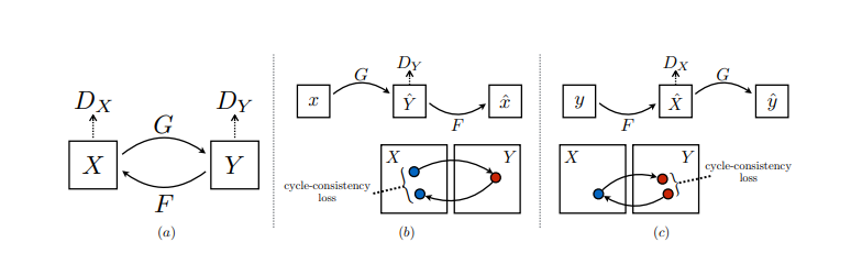
CycleGAN consists of two generators and two discriminators, allowing it to implement bi-directional mappings. During training, the first pair of generators and discriminators focus on the forward mapping from domain $A$ to domain $B$, while the second pair does the opposite.

The cycle-consistency loss, in particular, helps in training these generators with unpaired images from the domains. In practice, it forces the composition of two mappings (for instance, from A to B then B back to A) to recover the input, thereby preserving the input image's style and content.

The architecture of CycleGAN is more symmetric than other GANs:

• Two generators, each responsible for a mapping direction (e.g., from apples to oranges and vice versa)
• Two discriminators, one for each domain

This symmetry helps with the effectiveness of the cycle-consistency loss and ensures that both mappings are as accurate as possible.

Applications

• Image-to-Image Translation: CycleGANs can transform images from one domain to another.

• Neural Style Transfer: By training on sets of real images and artwork, CycleGANs have been used to transfer the style of art to real photographs.

• Data Augmentation: These models can generate new, realistic images for datasets, especially useful when working with limited data.

• Super-Resolution: Converting low-resolution images to high-resolution ones, a process called super-resolution.

• Domain Adaptation: Adapting models trained in one domain to work in another, unseen domain.

Code Example: CycleGAN with PyTorch

Here is the Python code:

import torch
import torch.nn as nn
import torch.optim as optim

# Define the two generators and discriminators
G_AB = Generator()
G_BA = Generator()
D_A = Discriminator()
D_B = Discriminator()

# Define loss functions
criterion_adv = nn.BCELoss()
criterion_cycle = nn.L1Loss()

# Define optimizers
optimizer_G = optim.Adam(itertools.chain(G_AB.parameters(), G_BA.parameters()), lr=lr, betas=(b1, b2))
optimizer_D_A = optim.Adam(D_A.parameters(), lr=lr, betas=(b1, b2))
optimizer_D_B = optim.Adam(D_B.parameters(), lr=lr, betas=(b1, b2))

# Training Loop
for epoch in range(num_epochs):
    for real_A, real_B in dataloader:
        real_A, real_B = real_A.to(device), real_B.to(device)

        # Adversarial Loss
        fake_B = G_AB(real_A)
        pred_real, pred_fake = D_B(real_B), D_B(fake_B)
        loss_GAN_AB = criterion_adv(pred_fake, torch.ones_like(pred_fake)) + criterion_adv(pred_real, torch.zeros_like(pred_real))
        
        # Cycle Consistency
        reconstructed_A = G_BA(fake_B)
        loss_cycle_A = criterion_cycle(reconstructed_A, real_A)

        # Update weights using the calculated losses and optimizers

15. Explain how GANs can be used for super-resolution imaging (SRGANs).

In the context of GANs, Super-Resolution GANs (SRGANs) are a specialized class of models designed to generate high-resolution images from low-resolution inputs.

Key Components

1. Generator (G): Transforms low-resolution images into high-resolution counterparts.
2. Discriminator (D): Differentiates between the generator's outputs and real high-resolution images.

Core Techniques

1. Adversarial Training: The generator and discriminator play a continuous game. The generator strives to fool the discriminator, while the discriminator aims to correctly classify real and fake images.

2. Perceptual Loss: Utilizes pre-trained networks (e.g., VGG) to ensure the generator produces perceptually realistic outputs.

3. Feature Pyramid Network (FPN): Augments the generator by incorporating a FPN architecture, enabling the generator to learn multi-scale representations.

4. PixelShuffle: Contains a sub-pixel convolutional layer that upscales feature maps, boosting the final image resolution.

5. Trained Discriminator: Uses pre-trained models to improve the discriminator's ability to distinguish between real and fake images.

Code Example: SRGAN

Here is the PyTorch code:

import torch
from torchvision import models
from torch import nn

# Load the VGG19 model
vgg = models.vgg19(pretrained=True).features
# Freeze its parameters
for param in vgg.parameters():
    param.requires_grad_(False)

# Define the Generator and Discriminator
class GeneratorSRGAN(nn.Module):
    def __init__(self):
        super(GeneratorSRGAN, self).__init__()
        # Define layers...
    
    def forward(self, x):
        # Implement forward pass...

class DiscriminatorSRGAN(nn.Module):
    def __init__(self):
        super(DiscriminatorSRGAN, self).__init__()
        # Define layers...
    
    def forward(self, x):
        # Implement forward pass...

# Instantiate the models
generator = GeneratorSRGAN()
discriminator = DiscriminatorSRGAN()

# Define the loss functions
adversarial_loss = nn.BCELoss()
perceptual_loss = nn.MSELoss()

# Define the optimizers
generator_optimizer = torch.optim.Adam(generator.parameters(), lr=0.0002, betas=(0.5, 0.999))
discriminator_optimizer = torch.optim.Adam(discriminator.parameters(), lr=0.0002, betas=(0.5, 0.999))

# Training loop
for epoch in range(num_epochs):
    for i, (low_res_images, high_res_images) in enumerate(dataloader):
        # Train the discriminator
        discriminator_optimizer.zero_grad()
        # ...

        # Train the generator
        generator_optimizer.zero_grad()
        # ...

        # Update the optimizers
        generator_optimizer.step()
        discriminator_optimizer.step()

# Generate a high-resolution image from a low-resolution input
fake_high_res_image = generator(low_res_input)

Explore all 52 answers here 👉 Devinterview.io - GANs