First, clone the repository to a local folder of your choosing.
Package requirements for installation can be found in requirements.txt or environment.yml.
To install requirements using pip, create a new virtual environment. Then run "pip install -r requirements.txt" with the virtual environment active and in the directory of the cloned repository.
See writeup for a more illustrative explanation.
See other writeup to see how I use neural networks to predict wave behavior using Torch.
See demo_simulation.ipynb for example use of the wavetorch.py module.
The wavetorch.py module allows you to simulate wave behavior with any amount of wave sources on a 2 dimensional grid. These wave sources can be customized as any mathematical function over time. For example, you may want to simulate the interference pattern between three different sine waves at varying frequencies in different locations.
Furthermore, parallelized computing via CUDA compatible GPU's is supported. With this module, you can generate your own rich datasets to test different methods of signal processing on. This is possible because of a machine learning module called Torch, which contains robust tensor manipulation tools.
Some mathematical implications for parallel processing on a GPU (for those of you familiar with the wave equation):
- The calculation of u may be parallelized across spatial coordinates x and y, i.e. use u(x,y,t) at all x and y to calculate u(x,y,t+dt)
- The calculation of u may not be parallelized across time, meaning we must know u(t) to predict u(t+dt)
At a high level, use the module as follows:
- Fill a dictionary with simulation metadata, including spacial and time resolution.
- Prepare a 2 dimensional tensor that shows what the wave medium looks like at start time.
- Prepare a list of dictionaries containing wave source coordinates, and their associated mathematical functions.
- Pass the objects created in steps 1-3, into the wavetorch.wave_eq function, which generates a dictioanry.
- Inside the generated dictionary is a 3d tensor containing the simulation data. I recommend saving it as a torch tensor ".pt" object using torch.save. You can also save it as an mp4 video to watch using imageio.mimwrite.
The module is located in the src folder:
- 'wavetorch.py' - module consisting of functions to simulate wave phenomena
Demos using the module for reference can be found in the demos folder:
- 'demo_simulation.ipynb' - Jupyter Notebook file showcasing how wavetorch.py can be used to generate a 2d video of wave phenomena, and the wave signal at different locations
- 'demo_signal_processing.ipynb' - Jupyter Notebook file showcasing how generated signals may be spectrally decomposed
The raw tensor file generated in this project has been ommited from the repository, due to its enourmous file size.
Wave Simulation at specific frame:

Wave Signal at different locations:


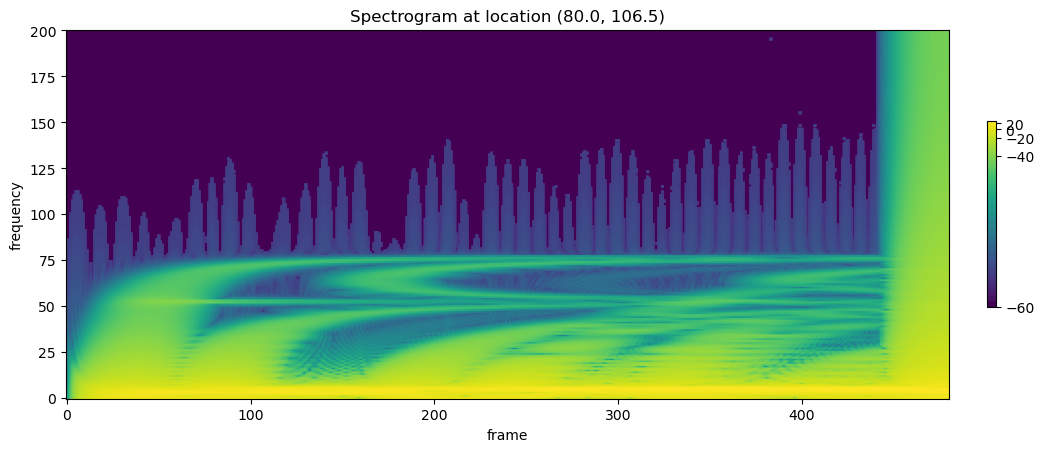
Spectrograms of wave at different locations:

Link to video of simulation of 2d waves over time:
https://www.youtube.com/watch?v=UdjUCrevOd0
I referenced Hans Petter Langtangen's works to understand computational physics as applied to partial differential equations. Please see the following link for more details:
http://hplgit.github.io/wavebc/doc/pub/._wavebc_cyborg004.html#sec:app:numerical