PyCont-Lite

PyCont-Lite is a lightweight, matrix-free arclength continuation library for solving nonlinear parametric systems

$$ G(u, p) = 0 $$

with automatic bifurcation detection, branch switching, and stability analysis.

Key Features

• Matrix-free: only need to implement $G(u, p)$, no Jacobians required.
• Adaptive continuation: robust predictor–corrector with adjustable step sizes.
• Bifurcation detection: automatically localizes and classifies folds and branch points.
• Branch switching: continues all discovered branches recursively.
• Stability analysis: computes leading eigenvalues to distinguish stable vs. unstable segments.
• Hopf Detection: detect and localize Hopf bifurcation points where the system changes from a steady state to period behavior (a limit cycle).
• Limit Cycle Continuation : Initialize the small-amplitude limit cycle around the Hopf point, and perform numerical continuation of this limit cycle.
• Lightweight plotting: quickly visualize bifurcation diagrams with plotBifurcationDiagram. Plots automatically distinguish stable vs. unstable branches.
• Structured output: branches (with stability) and events (folds, bifurcations) are returned for further analysis.

The main goal of PyCont-Lite is to provide a unified continuation and bifurcation toolkit for PDEs and neural models. We explicitly aim for a complete backend-agnostic implementation so PyCont-Lite can be used with numpy, PyTorch and Jax.

Installation & Requirements

PyCont-Lite requires only:

• numpy
• scipy
• matplotlib

Install via PyPI (pip):

pip install pycont-lite

Quick Examples

Pitchfork Bifurcation

import numpy as np
import pycont

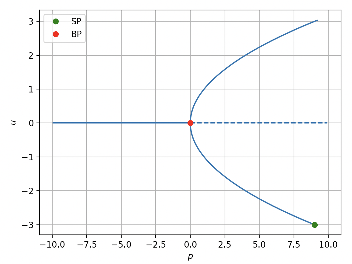
# Define the pitchfork function
def G(u, p):
    return u**3 - p*u

# Initial guess
u0 = np.array([-3.0])
p0 = 9.0

# Run continuation
ds_max = 0.01
ds_min = 1.e-6
ds = 0.001
n_steps = 1000
solver_parameters = {"tolerance": 1e-10}
continuation_result = pycont.arclengthContinuation(G, u0, p0, ds_min, ds_max, ds, n_steps, solver_parameters=solver_parameters)

# Plot the solution curve
pycont.plotBifurcationDiagram(continuation_result)

Fold Bifurcation

import numpy as np
import pycont

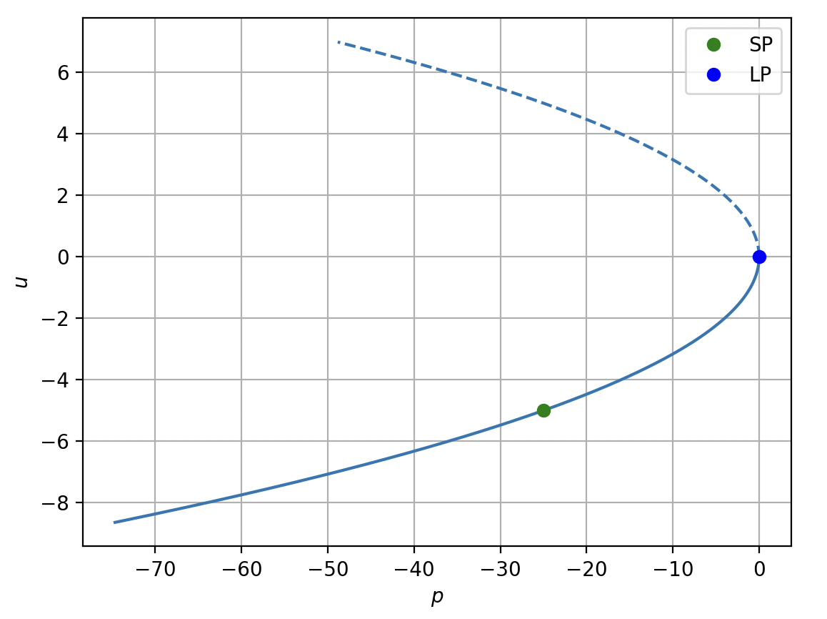
# Define the fold function
G = lambda x, r: r + x**2

# Initial guess
u0 = np.array([-5.0])
p0 = -u0[0]**2

# Run continuation
ds_max = 0.01
ds_min = 1.e-6
ds = 0.001
n_steps = 5000
solver_parameters = {"tolerance": 1e-10}
continuation_result = pycont.arclengthContinuation(G, u0, p0, ds_min, ds_max, ds, n_steps, solver_parameters=solver_parameters)

# Plot the curves
pycont.plotBifurcationDiagram(continuation_result)

Bratu: PDE Example

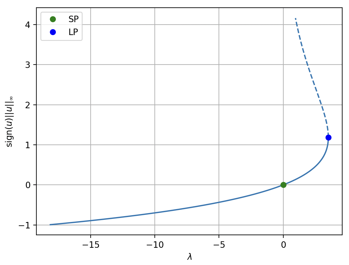
The nonlinear boundary value problem

$$ u_{xx} + \lambda e^u = 0, \quad u(0)=u(1)=0 $$

discretized with finite differences:

import numpy as np
import pycont

N = 101 # total number of points
x = np.linspace(0.0, 1.0, N)
dx = x[1] - x[0]

def G(u: np.ndarray, lam: float) -> np.ndarray:
    u_full = np.zeros(N, dtype=float)
    u_full[1:-1] = u
    
    u_xx = (u_full[:-2] - 2.0 * u_full[1:-1] + u_full[2:]) / (dx * dx)
    r = u_xx + lam * np.exp(u_full[1:-1])
    return r

# We know that u = 0 for lambda = 0 - otherwise we must solve G(u, lambda0) = 0.
lam0 = 0.0
u0 = np.zeros(N-2)

# Do continuation
ds_max = 0.01
ds_min = 1e-6
ds0 = 1e-4
n_steps = 2000
solver_parameters = {"tolerance": 1e-10}
continuation_result = pycont.arclengthContinuation(G, u0, lam0, ds_min, ds_max, ds0, n_steps, solver_parameters=solver_parameters)

# Plot the bifurcation diagram (lambda, max(u))
u_transform = lambda u : np.sign(u[50]) * np.max(np.abs(u))
pycont.plotBifurcationDiagram(continuation_result, u_transform=u_transform, p_label=r'$\lambda$', u_label=r'$\text{sign}(u) ||u||_{\infty}$')

This produces the classical S-shaped bifurcation curve with a fold near $\lambda \approx 3.51$.

Allen-Cahn

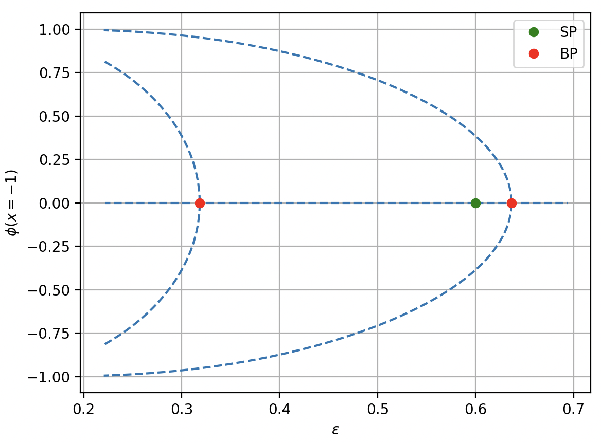
The nonlinear boundary value problem

$$ \varepsilon \phi_{xx} - \varepsilon^{-1} \phi \left(\phi^2 - 1\right) = 0, \quad \phi_x(-1) = \phi_x(1)=0 $$

discretized with finite differences:

import numpy as np
import pycont

N = 100
x = np.linspace(-1.0, 1.0, N)
dx = (x[-1] - x[0]) / (N-1)

def laplace_neumann(phi, dx):
    phi_ext = np.hstack([phi[1], phi, phi[-2]])
    phi_l = np.roll(phi_ext, -1)[1:-1]
    phi_r = np.roll(phi_ext,  1)[1:-1]
    return (phi_l - 2.0*phi + phi_r) / dx**2
def G(phi : np.ndarray, eps : float):
    phi_xx = laplace_neumann(phi, dx)
    rhs = eps * phi_xx - phi * (phi**2 - 1.0) / eps
    return rhs

# Initial Point
eps0 = 0.6
phi0 = np.zeros(N)

# Do continuation
tolerance = 1e-9
ds_max = 1e-2
ds_min = 1e-6
ds0 = 1e-4
n_steps = 1000
solver_parameters = {"tolerance" : tolerance, "param_min" : 0.22, "param_max" : 0.7}
continuation_result = pycont.arclengthContinuation(G, phi0, eps0, ds_min, ds_max, ds0, n_steps, solver_parameters=solver_parameters, verbosity='verbose')

# Plot the bifurcation diagram eps versus phi(x=-1)
u_transform = lambda phi: phi[0]
pycont.plotBifurcationDiagram(continuation_result, u_transform=u_transform, p_label=r'$\varepsilon$', u_label=r'$\phi(x=-1)$')

This reproduces the many bifurcation points as $\varepsilon \to 0$.

Hopf Bifurcation

Since version 0.4.0, PyCont-Lite is also able to detect Hopf bifurcations. A Hopf bifurcation occurs when two complex-conjugated eigenvalues of the Jacobian $G_u(u,p)$ cross the imaginary axis. The prototypical example is the Hopf normal form

$$ \begin{align} \mu x - y - (x^2 + y^2) x &= 0 \\ x - \mu y - (x^2 + y^2) y &= 0 \\ \end{align} $$

which has a Hopf point at $(x,y) = (0,0)$ with $\mu = 0$. PyCont-Lite can find this Hopf bifurcation point (see examples/NormalHopf.py):

import numpy as np
import pycont

def G(u : np.ndarray, mu : float) -> np.ndarray:
    x = u[0]; y = u[1]
    Gx = mu*x - y - (x**2 + y**2) * x
    Gy = x + mu*y - (x**2 + y**2) * y
    return np.array([Gx, Gy])
mu0 = -1.0
u0 = np.array([0.0, 0.0])

ds_max = 0.01
ds_min = 1.e-6
ds = 0.01
n_steps = 200
solver_parameters = {"tolerance": 1e-10, 'hopf_detection' : True}
continuation_result = pycont.arclengthContinuation(G, u0, mu0, ds_min, ds_max, ds, n_steps, solver_parameters)

pycont.plotBifurcationDiagram(continuation_result, p_label=r'$\mu$')

which produces the (trivial) bifurcation diagram

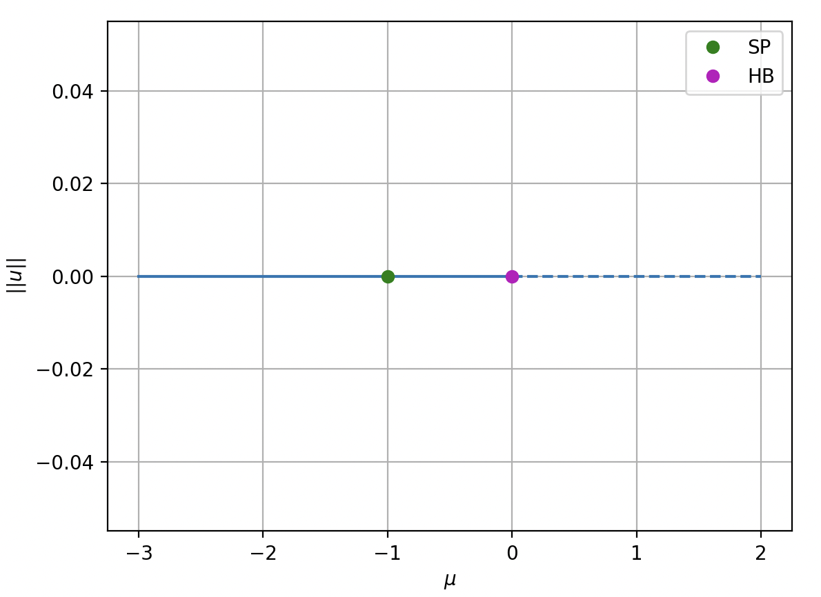
For now, Hopf bifurcation detection is disabled by default, so the user must supply it via 'hopf_detection' : True in the solver parameters.

Since version 0.6.0, PyCont-Lite can also perform limit cycle computations and continuation. The limit cylces for the Normal Hopf example are concentric circles.

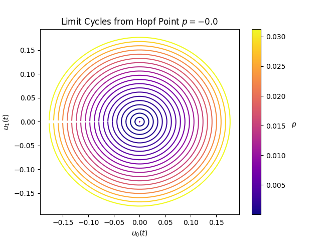
Limit cycle continuation is enabled whenever Hopf detection is enabled. Users can opt out of limit cycle coninuation via the 'limit_cycle_continuation' : False flag in the solver parameters.

The Brusselator

A classical yet chemically important system that has Hopf and limit-cyle dynamics is the Brusselator (see examples/Brusselator.py).

$$ \begin{align} A - (B+1) x + x^2 y &= 0 \\ B x - x^2 y &= 0 \\ \end{align} $$

For $A = 1$, this system has a Hopf bifurcation at $B = 1$

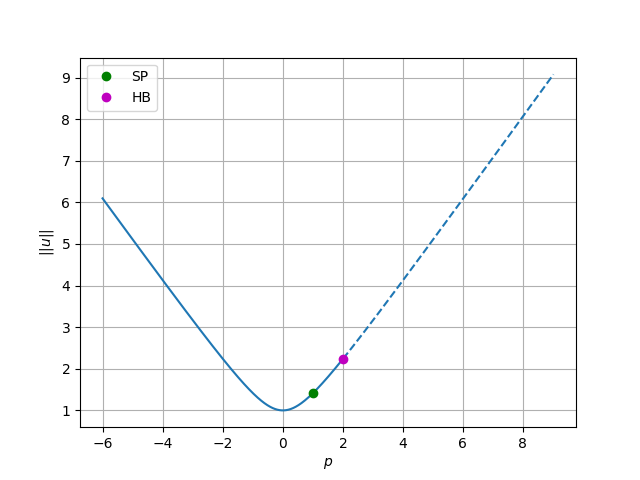
and the limit cycles initially look elliptic

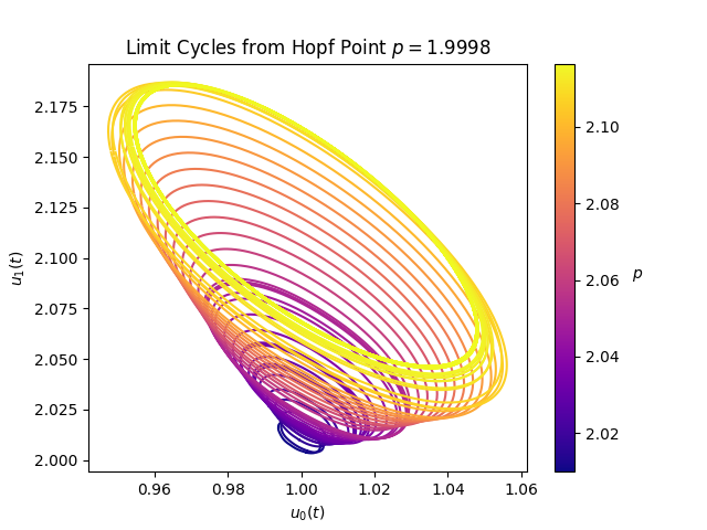
Both the bifurcation diagram and small-amplitude limit cylces have been computed using PyCont-Lite.

Advanced Hopf Example: The Fitzhugh-Nagumo Equations

For a more interesting system that exhibits a Hopf bifurcation, consider the Fitzhugh-Nagumo equations

$$ \begin{align} u_{xx} + u - u^3 - v = 0 \\ \delta v_{xx} + \varepsilon \left(u - a_1 v - a_0\right) = 0 \end{align} $$

with $\delta = 4$, $a_1 = 2$ and $a_0 = -0.03$. This system exhibits a Hopf bifurcation point near $\varepsilon \approx 0.018$, and a fold point near $\varepsilon \approx 0.94$. See examples/FitzhughNagumoPDEs.py for the code:

N = 100
L = 20.0
x = np.linspace(0.0, L, N)
dx = L / (N-1)

# Build the FHN objective function through finite differences
a0 = -0.03
a1 = 2.0
delta = 4.0
def G(z : np.ndarray, eps : float):
    u, v = z[:N], z[N:]
    u_xx = laplace_neumann(u, dx)
    v_xx = laplace_neumann(v, dx)
    u_rhs = u_xx + u - u**3 - v
    v_rhs = delta * v_xx + eps * (u - a1*v - a0)
    return np.concatenate((u_rhs, v_rhs))

# Do continuation.
tolerance = 1e-9
ds_max = 0.01
ds_min = 1e-6
ds0 = 1e-3
n_steps = 1000
solver_parameters = {"tolerance" : tolerance, "param_min" : 0.01, "hopf_detection" : True}
continuation_result = pycont.arclengthContinuation(G, z0, eps0, ds_min, ds_max, ds0, n_steps, solver_parameters)

# Plot the bifurcation diagram `eps` versus <u>
u_transform = lambda z: np.average(z[:N])
pycont.plotBifurcationDiagram(continuation_result, u_transform=u_transform, p_label=r'$\varepsilon$', u_label=r'$<u>$')

Note that we limit exploration to a minimal parameter value of $\varepsilon = 0.01$ for plotting purposes. PyCont-Lite detects the fold and Hopf points nicely

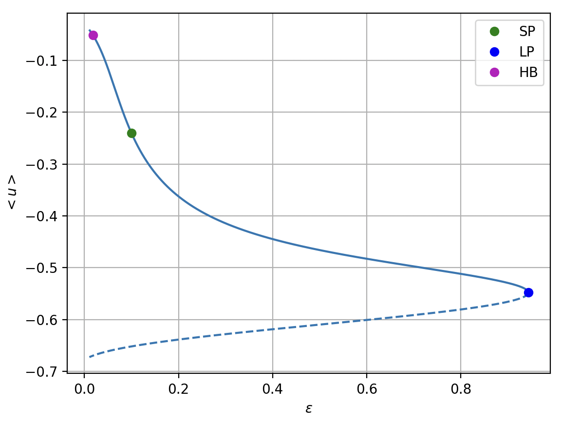
limit cycle calculations are very expensive for high-dimensional systems, so we do not show them here.

Plotting Bifurcation Diagrams

PyCont-Lite includes a helper function plotBifurcationDiagram for quick visualization. Stable segments are shown as solid lines and unstable segments as dashed lines, just like in AUTO/MATCONT. By default, it plots the parameter value on the horizontal axis and the transformed state variable on the vertical axis.

import pycont

# After running continuation...
pycont.plotBifurcationDiagram(continuation_result)

For multi-dimensional systems, you can specify how to reduce $u$ to a single scalar for plotting via the u_transform argument.

• Default behavior:
  • If $u$ has dimension 1 → plot $u$ directly.
  • If $u$ has dimension >1 → plot the Euclidean norm $||u||$.
• Custom transform (example: plot the maximum component of $u$):

pycont.plotBifurcationDiagram(result, u_transform=lambda u: u.max())

Solver Parameters

You can fine-tune the solver by passing a dictionary:

solver_parameters = {
    "rdiff": 6e-6,              # central finite-difference step
    "nk_maxiter": 20,           # Newton-Krylov iterations
    "tolerance": 1e-10,         # nonlinear tolerance
    "bifurcation_detection": True,
    "analyze_stability": True,  # compute leading eigenvalue
    "initial_directions": "both"  # 'both', 'increase_p', 'decrease_p'
}

A full list of options can be found in the documentation of the main arclengthContinuation function.

Verbosity Options

Control how much progress info PyCont-Lite prints during continuation. Three levels are supported:

Level	What you see
off	No progress messages (errors only).
info	One-line progress per step + event summaries (recommended default).
verbose	Solver details: Newton–Krylov iterations, step rejections, preconditioner notes.

Pass the level to arclengthContinuation via the verbosity argument. You can use a string (case-insensitive) or the enum:

from pycont import arclengthContinuation, Verbosity

# String (case-insensitive)
arclengthContinuation(G, u0, p0, ..., verbosity="info")

# Enum
arclengthContinuation(G, u0, p0, ..., verbosity=Verbosity.VERBOSE)

Default is info. See the Allen–Cahn example above for a typical verbose run.

Output Format

arclengthContinuation returns a ContinuationResult object with:

• branches: list of Branch objects (u_path, p_path, stability flag, etc.)
• events: list of Event objects (start points, folds, bifurcations)

This makes it easy to explore and plot bifurcation diagrams programmatically.

Planned Features

The following features are under active consideration for future releases:

• Complete backend-agnostic implementation
• Choice between finite-differences and explicit user-specified Jacobians
• Features for external automatic differentiation for gradients.

License

This project is licensed under the MIT License — see the LICENSE file for details.

Acknowledgement

I started this project because most continuation software is either legacy Fortran (AUTO), Matlab-only (MATCONT, COCO), or heavyweight. PyCont-Lite is meant to be modern, lightweight, and useful both for industry and academia!

For feature requests or contributions, feel free to open an issue or reach out: hannesvdc[at]gmail[dot]com.