R package for Skeleton-based Analysis Methods
skeletonMethods is R package implementing the Skeleton Clustering and Skeleton Clustering methods in :
Zeyu Wei, and Yen-Chi Chen. "Skeleton Clustering: Dimension-Free Density-based Clustering." 2021. Zeyu Wei, and Yen-Chi Chen. "Skeleton Regression." 2021.
The manuscript of the paper can be found at here.
The package currently only exists on github. Installed directly from this repo with help from the devtools package. Run the following in R:
```R
install.packages("devtools")
devtools::install_github("JerryBubble/skeletonMethods")
```
The package is actively developing.
The follwoing figure illustrates the overall procedure of the skeleton clustering method.
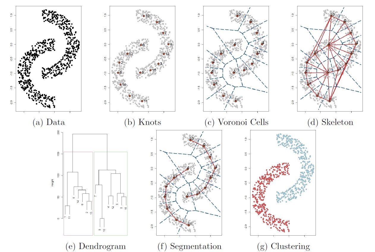
Starting with a collection of observations (panel (a)),
we first find knots, the representative points of the entire data (panel (b)). By default we use the k-means algorithm to choose knots.
Then we compute the corresponding Voronoi cells induced by the knots (panel (c))
and the edges associating the Voronoi cells (panel (d), this is the Delaunay triangulation).
For each edge in the graph, we compute a density-based similarity measure that quantifies the closeness of each pair of knots.
For the next step we segment knots into groups based on a linkage criterion (single linkage in this example), leading to the dendrogram in panel (e).
Finally, we choose a threshold that cuts the dendrogram into
Check out this page for animations on the skeleton framework.
Load R-package and simulate Yinyang data of dimension 100
library("skeletonMethods")

dat = Yinyang_data(d = 100)
X0 = dat$data
y0 = dat$clus
Other simulation data used in the skeleton clustering paper can be genereted similarly: Mickey_data() for Mickey data, MM_data() for Manifold Mixture data, MixMickey_data() for Mix Mickey data, MixStar_data() for mixture of three Gaussian cluster giving a star shape, and ring_data() for Ring data
Also, with set.seed(1234) the 1000-dimensional simulated datasets are also built into the skeletonClus package, with names Yinyang1000, Ring1000, Mickey1000, MixMickey1000, MixStar1000, ManifoldMix1000. Those built in datasets can be load into R working environment by
data(Yinyang1000)We proceed with constructing the weighted skeleton with overfitting k-means, wihch can be donw with the skeletonCons function:
skeleton = skeletonCons(X0, rep = 1000)For more flexible usage of skeletonCons see the help page at
?skeletonConsThe knots and the Voronoi density edge weights can be accessed as
skeleton$centers
skeleton$voron_weights
The Face density, Tube density, and Average Distance density weights can be accessed in similar fashion. We then segment the knots based on the edge weights with hierarchical clustering (taking Voronoi density for example):
##turn similarity into distance
VD_tmp = max(skeleton$voron_weights) - skeleton$voron_weights
diag(VD_tmp) = 0
VD_tmp = as.dist(VD_tmp)

##perform hierarchical clustering on the distance matrix
VD_hclust = hclust(VD_tmp, method="single")
If the final number of clusters is unknown, we can plot the dendrogram of hierarchical clustering to see the structure of the data and pick a cutting threshold. Here we know the data have 5 components and hence we cut the tree into 5 groups.
##plot dendrogram
plot(VD_hclust)
##cut tree
VD_lab = cutree(VD_hclust, k=5)
Then we assign the label of each observation to have the same group membership as the closest knot
X_lab_VD = VD_lab[skeleton$cluster]With the mclust R package we can calculate the adjusted Rand index:
library("mclust")
voron_rand = adjustedRandIndex(X_lab_VD, y0)
FInally we can get a plot to visualize the clustering result:
plot(X0[,1], X0[,2], col = cols[X_lab_VD], main = "Skeleton Clustering with Voronoi Density", xlab = "X", ylab = "Y", cex.main=1.5)Like in the skeleton clustering framework, for regression puporse we also first construct a skeleton graph to represent the covariates. Particularly, for regression we use the density-aided similarity measure called Voronoi density to help cut skeleton if needed, and such construction can be done with the function voronSkeleton. Then we project the data covariates onto the skeleton graph with function skelProject and compute the skeleton-based distances between them with function dskeleton. Then we implement different non-parametric regression techiniques on the skeleton graph:
Let skelKernel fits this regressor.
First, we construct a linear model on each edge of the graph while requiring the predicted values to agree on shared vertices. For the fitting process, note that the linear model on each edge is determined by the values on the two connected vertices, and we transform the covariate and use ordinary least squares to fit the model, with the coefficients representing values on the knots. The function skelLinear fits this linear spline model.
Higher order splines, which require higher-order smoothness on the knots, can also be fit, but users should be cautious with the directions of the derivatives. skelQuadratic and skelCubic fit quadratic and cubic spline respectively.
We can use skeleton distances to search for neighbors and implement the classical kNN regression technique. This is implemented in function skelknn.
skelReg_runAll function performs prediction on test dataset with all the skeleton-based functions, and users can specify a sequence of parameters for the different methods. For example
d = 100 #dimension of covariates
set.seed(1234)
data = Yinyang_reg_data(d = d) #simulate the Yinyang Regression data example
X0  = as.matrix(data$data)
Y0  = data$Y
trainID = sample(nrow(X0),nrow(X0)*0.75)
trainX = X0[trainID,]
trainY = Y0[trainID]
testX = X0[-trainID,]
testY = Y0[-trainID]
fits = skelReg_runAll(trainX,trainY,testX, seed = NULL,
                      hrate_seq = c(1,2),
                      k_seq = seq(3,6, by=3),
                      numknots=NULL,
                      k_cut=5,
                      rep = 1000)
skelReg_runAllCV function performs cross-validation with all the skeleton-based functions, and users can specify a sequence of parameters to test on. For example
d = 100 #dimension of covariates
set.seed(1234)
traindata = Yinyang_reg_data(d = d) #simulate the Yinyang Regression data example
X0  = as.matrix(traindata$data)
Y0  = traindata$Y
results = skelReg_runAllCV(X0,Y0, seed = NULL, nfold = 2,
                                    hrate_seq = c(1,2),
                                    k_seq = c(3,6),
                                    numknots=NULL,
                                    k_cut=5,
                                    rep = 1000)
In addition to the two wrapper functions that run all the methods together, each step in the regression framework is also implemented and users can run them step-by-step to gain better control over the regression methods. An detailed example run with the steps are presented belwo.
library("skeletonMethods")
d = 100 #dimension of covariates
set.seed(1234)
traindata = Yinyang_reg_data(d = d) #simulate the Yinyang Regression data example
X0  = as.matrix(traindata$data)
Y0  = traindata$Y

#split the data for cross validation
set.seed(1234)
nfold = 5
n = length(Y0)
fsplit = c(rep( floor(n/nfold), nfold-1), n - floor(n/nfold)*(nfold-1))
folds = split(1:nrow(X0), sample(rep(1:nfold, fsplit)))

#loop for optimal bandwidth rate
hrate_seq = c(1/8, 1/4,1/2,1,2,4,6, 8,10,12, 14,16)
#loop for knn reg k
k_seq = seq(3,36, by=3)
#choices for number of knots
ntrain = nrow(X0)*(nfold-1)/nfold
numknots_seq = round(sqrt(ntrain)*c(0.25,0.5,0.75,1,1.25,1.5,1.75,2,4,8))
iknot = 4 #here we use the rule of thumb for number of knots

####################
#Allocate space for saving results
####################
skelResults = matrix(nrow = (nfold*length(hrate_seq)), ncol = 3)#skeleton kernel regression with adaptive bandwidth
skelResults2 = matrix(nrow = (nfold*length(hrate_seq)), ncol = 3)#skeleton kernel regression with global bandwidth
skelnnResults = matrix(nrow = (nfold*length(k_seq)), ncol = 3)#skeleton kNN regressor
knnResults = matrix(nrow = (nfold*length(k_seq)), ncol = 3) #classical kNN regressor for comparison
lsplineResults = matrix(nrow = nfold, ncol = 2) #skeleton linear spline
qsplineResults = matrix(nrow = nfold, ncol = 2) #skeleton quadratic spline
csplineResults = matrix(nrow = nfold, ncol = 2) #skeleton cubic spline

skelpred = list()
for (j in 1:length(hrate_seq)) {
  skelpred[[j]] = rep(NA,n)
}
skelpred2 = list()
for (j in 1:length(hrate_seq)) {
  skelpred2[[j]] = rep(NA,n)
}
skelnnpred = list()
for (j in 1:length(k_seq)) {
  skelnnpred[[j]] = rep(NA,n)
}
knnpred = list()
for (j in 1:length(k_seq)) {
  knnpred[[j]] = rep(NA,n)
}
lsplinefit = rep(NA,n)
qsplinefit = rep(NA,n)
csplinefit = rep(NA,n)

################################################################################
#Perform cross validation
################################################################################
for(ifold in 1:nfold){

  testIndexes = folds[[ifold]]
  testX = X0[testIndexes, ,drop = FALSE]
  trainX = X0[-testIndexes, ]
  testY = Y0[testIndexes,drop = FALSE]
  trainY = Y0[-testIndexes]

  ######
  #construct skeleton
  #####
  numknots = numknots_seq[iknot] #number of knots
  voronSkel = voronSkeleton(trainX,numknots = numknots, k_cut = 5, rep=1000, seed=1234)
  centers = voronSkel$centers
  labels = voronSkel$labels
  kdists = voronSkel$kdists
  edgedists = voronSkel$edgedists
  g = voronSkel$g
  nn = voronSkel$nn

  #####
  #calculate the projection for training data point
  ######
  px = skelProject(nn = nn, X = trainX, skeleton = voronSkel)

  #####
  #situate test observations on the graph
  #####
  newnn = RANN::nn2(centers, testX, k=2)$nn.idx
  #calculate the projection for new data points
  newpx = skelProject(nn = newnn, X = testX, skeleton = voronSkel)

  #graph distances between test observations and training points
  testSkeldists = matrix(Inf,nrow = nrow(testX), ncol = nrow(trainX))
  for (i in 1:nrow(testX)) {
    #calculate graph distances between new obs and sample points
    for (j in 1:nrow(trainX)) {
      if(length(intersect(newnn[i,], nn[j,]))>0){ #only calculate distance between nearby data points
        testSkeldists[i,j] = dskeleton(nn[j,], newnn[i,], px[j], newpx[i], voronSkel)
      }
    }
  }

  #######
  #S-kernel regression with global bandwidth
  #######
  #calculate the based bandwidth for cross validation
  centerband = skelBand(centernn = NULL, px = px, skeleton = voronSkel)
  testfit_tmp2 = numeric(nrow(testX))
  for (ihrate in 1:length(hrate_seq)) {
    hrate_tmp = hrate_seq[ihrate]
    h1 = centerband*hrate_tmp
    #regression on test data
    testfit_tmp2 = skelKernel(h1, testX,testSkeldists, trainY)
    skelpred2[[ihrate]][testIndexes] = testfit_tmp2
    skelResults2[(ihrate-1)*nfold+ifold,1] = sum((testfit_tmp2 - testY)^2)
    skelResults2[(ihrate-1)*nfold+ifold,2] = hrate_tmp
    skelResults2[(ihrate-1)*nfold+ifold,3] = ifold

  }

  #######
  #S-kernel regression with varying bandwidth
  #######
  testfit_tmp = numeric(nrow(testX))
  for (ihrate in 1:length(hrate_seq)) {
    hrate_tmp = hrate_seq[ihrate]
    #regression on test data
    testfit_tmp = skelKerneladopt(hrate_tmp, testX,testSkeldists, trainY)
    skelpred[[ihrate]][testIndexes] = testfit_tmp
    skelResults[(ihrate-1)*nfold+ifold,1] = sum((testfit_tmp - testY)^2)
    skelResults[(ihrate-1)*nfold+ifold,2] = hrate_tmp
    skelResults[(ihrate-1)*nfold+ifold,3] = ifold

  }

  ######
  #S-kNN regressor, using graph distance for kNN
  ######
  gnntestfit_tmp = numeric(nrow(testX))
  for (ik in 1:length(k_seq)) {
    k_tmp = k_seq[ik]
    #fit on test data
    gnntestfit_tmp = skelknn(k_tmp, testX,testSkeldists, trainY)
    skelnnpred[[ik]][testIndexes] = gnntestfit_tmp
    skelnnResults[(ik-1)*nfold+ifold,1] = sum((gnntestfit_tmp - testY)^2)
    skelnnResults[(ik-1)*nfold+ifold,2] = k_tmp
    skelnnResults[(ik-1)*nfold+ifold,3] = ifold

  }

  ######
  #classical kNN regression for comparison
  #####
  knntestfit_tmp = numeric(nrow(testX))
  #use knn reg
  for (ik in 1:length(k_seq)) {
    k_tmp = k_seq[ik]
    knnTestFit = FNN::knn.reg(trainX, test = testX, trainY, k = k_tmp)
    knnpred[[ik]][testIndexes] = knnTestFit$pred
    knnResults[(ik-1)*nfold+ifold,1] = sum((knnTestFit$pred- testY)^2)
    knnResults[(ik-1)*nfold+ifold,2] = k_tmp
    knnResults[(ik-1)*nfold+ifold,3] = ifold
  }

  ######
  #linear spline on graph with closed-form solution
  ######
  slinearmodel = skelLinear(newnn, newpx,  px, trainY, voronSkel)
  trainZ = slinearmodel$trainZ  #modified data matrix for training data from projection
  testZ = slinearmodel$testZ   #modified data matrix for test data from projection
  lmod = slinearmodel$model #the model
  lmpred = slinearmodel$pred #the predicted values
  lsplinefit[testIndexes] =  lmpred
  lsplineResults[ifold,1] = sum((testY -lmpred)^2)
  lsplineResults[ifold,2] = ifold

  ######
  #quadratic spline on graph with closed-form solution
  ######
  squadraticmodel = skelQuadratic(newnn, newpx,  px, trainY, voronSkel)
  trainZ = squadraticmodel$trainZ
  testZ = squadraticmodel$testZ
  lmod2 = squadraticmodel$model
  lmpred2 = squadraticmodel$pred
  qsplinefit[testIndexes] =  lmpred2
  qsplineResults[ifold,1] = sum((testY -lmpred2)^2)

  ######
  #cubic spline on general graph with closed-form solution (2p+1 polynomial)
  ######
  scubicmodel = skelCubic(newnn, newpx,  px, trainY, voronSkel)
  trainZ = scubicmodel$trainZ
  testZ = scubicmodel$testZ
  lmod3 = scubicmodel$model
  lmpred3 = scubicmodel$pred
  csplinefit[testIndexes] =  lmpred3
  csplineResults[ifold,1] = sum((testY -lmpred3)^2)
  csplineResults[ifold,2] = ifold

}### end cross validation

library(dplyr)
skelSSE = as.data.frame(skelResults) %>% group_by(V2) %>% summarise(skelSSE = sum(V1))
names(skelSSE)[1] = "bandrate"

skelSSE2 = as.data.frame(skelResults2) %>% group_by(V2) %>% summarise(skelSSE2 = sum(V1))
names(skelSSE2)[1] = "bandrate"

knnSSE = as.data.frame(knnResults) %>% group_by(V2) %>% summarise(knnSSE = sum(V1))
names(knnSSE)[1] = "nneighbor"

skelknnSSE = as.data.frame(skelnnResults) %>% group_by(V2) %>% summarise(skelknnSSE = sum(V1))
names(skelknnSSE)[1] = "nneighbor"

SSEresults = list(skelSSE= as.data.frame(skelSSE),
                  skelSSE2= as.data.frame(skelSSE2),
                  knnSSE=as.data.frame(knnSSE),
                  skelknnSSE=as.data.frame(skelknnSSE),
                  lsplineSSE = sum(lsplineResults[,1]),
                  qsplineSSE = sum(qsplineResults[,1]),
                  csplineSSE = sum(csplineResults[,1])
)
fits = list(skelpred= skelpred,
            skelpred2= skelpred2,
            knnpred= knnpred,
            skelnnpred= skelnnpred,
            lsplinefit= lsplinefit,
            qsplinefit= qsplinefit,
            csplinefit= csplinefit
)