FAQ

Short answers to the questions that come up in the first days with the package, with links to the pages and to the sections of the manual that say more. The code on this page runs in one session, from the top: the second answer declares the electron gas, which the later ones use.

Which function gives the object I need?

The objects of a calculation are derivatives of a few generating functionals (Z, log Z, the Luttinger–Ward functional Φ, the effective actions), and the package computes them as such; the functions named after the objects are shortcuts that give the same results. For the electron gas of the README (Z0, interaction, the propagator G0 made full as G):

object	what it is	function
Green function G(x, y) = −⟨T ψ(x) ψ̄(y)⟩	a derivative of Z with respect to η̄(x) and η(y)	-PerturbativeCorrelationFunction[Z0, {psi[x], psibar[y]}, interaction, n]
connected functions	derivatives of log Z	ConnectedCorrelationFunction[Z0, {psi[x1], psibar[x2], ...}, interaction, n]
connected vacuum diagrams	log(Z/Z₀)	ConnectedVacuumDiagrams[Z0, interaction, n]
Luttinger–Ward functional Φ[G]	minus the 2PI vacuum diagrams, with G₀ → G	LuttingerWardFunctional[Z0, interaction, n, G0 -> G]
self-energy Σ(x, y)	δΦ/δG(y, x): FunctionalDerivative[Phi, G[y, x]]	SelfEnergy[Phi, G, {x, y}]
irreducible vertex Γ⁰(x₁, x₂; x₃, x₄)	δ²Φ/δG(x₄, x₃)δG(x₂, x₁): FunctionalDerivative[Phi, G[x4, x3], G[x2, x1]]	IrreducibleVertex[Phi, G, {x1, x2, x3, x4}]
1PI effective action Γ[Ψ̄, Ψ]	the Legendre transform of −log Z with respect to η and η̄: S[Ψ̄, Ψ] − ½ Tr ln(−S''[Ψ̄, Ψ]) + Γ₁[Ψ̄, Ψ]	EffectiveAction1PI[Z0, interaction, n, {psi -> Psi, psibar -> Psibar}, G0 -> G0]
full vertex F(x₁, x₂; x₃, x₄)	the fourth derivative of the 1PI action with respect to the means	PerturbativeFullVertex[Z0, interaction, n, {psi, psibar}, {x1, x2, x3, x4}, G0 -> G]
vertex of the density Λ(x₁, x₂; z)	−δG⁻¹(x₁, x₂)/δU(z), U coupled to the density	PerturbativeDensityVertex[Z0, interaction, n, {psi, psibar}, {x1, x2, z}, G0 -> G]
2PI effective action Γ[G]	the Legendre transform of −log Z with respect to the two-point source: Φ[G] − Tr ln(−G⁻¹) − Tr(G₀⁻¹G − 1)	EffectiveAction2PI[Phi, G0 -> G]

The effective actions, with their notation (S the classical action, S'' its second derivative, Γ₁ and Γ₂), are in Conventions. The map of the functions places every public name by its role in a calculation, and ?Name gives its usage message.

What is the difference between PerturbativeCorrelationFunction and ConnectedCorrelationFunction?

PerturbativeCorrelationFunction is the expectation value ⟨…⟩ = ⟨… e^(−S_int)⟩₀/⟨e^(−S_int)⟩₀: the vacuum bubbles cancel, but a function of four or more fields keeps its disconnected terms. ConnectedCorrelationFunction is the cumulant, the derivative of log Z, with only the diagrams in which all the external points are connected. The four-point function of free fermions (order 0):

Needs["FunctionalDiagrams`"]
DeclareGrassmannSource[eta, etabar];
DeclareField[psi, etabar]; DeclareField[psibar, eta, -1];
Z0 = Exp[-IntegralOver[G0[x, y] etabar[x] ** eta[y], {x, y}]];
DeclareSymmetric[V]; DeclareInteractionLine[V]; DeclareDirectedPropagator[G0];
interaction =
  1/2 IntegralOver[V[x, y] psibar[x] ** psibar[y] ** psi[y] ** psi[x], {x, y}];
fields = {psi[x1], psibar[x2], psi[x3], psibar[x4]};
PerturbativeCorrelationFunction[Z0, fields, interaction, 0]
ConnectedCorrelationFunction[Z0, fields, interaction, 0]

-(G0[x1, x4] G0[x3, x2]) + G0[x1, x2] G0[x3, x4]
0

For the Green function, a function of two fields, the two are the same.

Why does a name like C or D fail?

The symbols built into the Wolfram Language have definitions of their own, which act before those of the package: D[x, y] is a derivative, and it is zero.

D[x, y]
DeclareSymmetric[D];

0
FunctionalDiagrams::builtin: D is a built-in symbol of the Wolfram Language, whose own definitions interfere with the package: use another name.

The package warns when a declaration names a built-in symbol. The usual ones to avoid are C, D, E, I, K, N, O, Beta, Gamma and GreenFunction; use names that are not built in, such as D0 or Dph for a phonon propagator and Q for a symmetric kernel. Context[name] is "System`" for a built-in symbol.

Why is a derivative zero?

FunctionalDerivative differentiates only with respect to declared sources (and to two-index kernels such as G[x, y], which need no declaration):

FunctionalDerivative[J[x] J[y], J[z]]

FunctionalDerivative::nosource: J[z] is not a declared source (DeclareSource, DeclareGrassmannSource): the derivative with respect to it is 0.
0

Declare the source first:

DeclareSource[J];
FunctionalDerivative[J[x] J[y], J[z]]

DeltaFunction[y, z] J[x] + DeltaFunction[x, z] J[y]

Why must Grassmann factors be multiplied with **?

Times sorts its factors, so that their order, and with it the sign of a product of Grassmann-odd factors, is lost. The package refuses such a product and stops the evaluation:

FunctionalDerivative[etabar[x] eta[y], eta[z], etabar[w]]

FunctionalDerivative::times: Grassmann-odd factors are multiplied with Times in eta[y] etabar[x]: Times sorts its factors, so that their order and the sign are lost. Write the product with ** ; the evaluation is aborted.
$Aborted

The message shows the factors as Times has already sorted them.

With ** the order is kept, and the derivatives, from the left and the rightmost first, give the signs:

FunctionalDerivative[etabar[x] ** eta[y], eta[z], etabar[w]]
FunctionalDerivative[etabar[x] ** eta[y], etabar[w], eta[z]]

DeltaFunction[w, x] DeltaFunction[y, z]
-(DeltaFunction[w, x] DeltaFunction[y, z])

Why do two equal results look different?

The functions of the package give their results in canonical form, with the internal points renamed z1, z2, ... by a canonical labelling: the names do not follow the order in which you wrote the points, and an expression you build yourself is in canonical form only after SimplifyDiagrams. Compare two results with SimplifyDiagrams[a - b], which is 0 exactly when they are the same sum of diagrams; see Orders and simplification.

Why is my diagram drawn with plain lines?

The pictures draw what the declarations say: an arrow for a propagator declared with DeclareDirectedPropagator, a wavy line for DeclareInteractionLine, a dashed one for DeclareLineStyle[h, "Dashed"], and so on. A two-label factor that is not declared is a plain line, and a factor of three or more labels a small hatched disc (a vertex function VertexFunction a cross-hatched one):

fock = IntegralOver[Gx[x, u] Vx[u, v] Gx[u, v] Gx[v, y], {u, v}];
DiagramPlot[fock, {x, y}]

DeclareDirectedPropagator[Gx]; DeclareInteractionLine[Vx];
DiagramPlot[fock, {x, y}]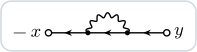

The weight changed as well: an interaction line stands for −V (see Reading the weights). For one picture only, the options "Directed" -> {Gx} and "Interactions" -> {Vx} do the same as the declarations. See Declaring a theory.

How do I set an option for the whole session?

Options are rules after the arguments. Options[f] gives those of a function with their defaults, and SetOptions changes a default until you change it back. With "CouplingOrder" -> {V, 2} the connected vacuum diagrams are those of order V² only:

Options[ConnectedVacuumDiagrams]
SetOptions[ConnectedVacuumDiagrams, "CouplingOrder" -> {V, 2}];
Length[DiagramTerms[ConnectedVacuumDiagrams[Z0, interaction, 3]]]
SetOptions[ConnectedVacuumDiagrams, "CouplingOrder" -> None];

{Method -> Automatic, CouplingOrder -> None}
5

A name that the function does not know, a misprint for instance, gives a message and is ignored, so that it never changes a result unnoticed:

ConnectedVacuumDiagrams[Z0, interaction, 2, "CoupligOrder" -> {V, 2}] ===
 ConnectedVacuumDiagrams[Z0, interaction, 2]

FunctionalDiagrams::optx: Unknown option CoupligOrder of ConnectedVacuumDiagrams, ignored; the options are {Method, CouplingOrder}.
True

How high an order can I compute?

The numbers of diagrams grow quickly, and the package is fast enough for the orders at which one can still look at them. The Green function of the electron gas at fourth order:

green4 = -PerturbativeCorrelationFunction[Z0, {psi[x], psibar[y]}, interaction, {4}];
Length[DiagramTerms[green4]]

706

This takes about a second; the fifth order (8162 diagrams) about twenty seconds. The showcase writes the time of each of its steps in Showcase/figures/values.txt. Compute only the orders you need: Orders and simplification.

Does the package do the momentum integrals?

In part. EvaluateMatsubara writes a diagram in momentum and Matsubara frequency, does the frequency sums and leaves the momentum integrals as MomentumSum; IntegrateLoops does the loop integrals that reduce to one-loop ones in dimensional regularization, and IntegrateOneLoop the one-loop integrals of QED. Anything beyond that is better done with a program made for loop integrals, from the integrands that the package writes. See Evaluating diagrams.

I changed the package, or installed a new version, and nothing changed

Needs does nothing when the package is already loaded. Load it again with Get, or start a new session: see Installation.

How do I cite the package?

As described in CITATION.cff; GitHub shows a Cite this repository button on the page of the repository, and the README gives a BibTeX entry.

Where do I report a problem?

In the issues of the repository, with $FunctionalDiagramsVersion, $Version, a short input that shows the problem (from Needs["FunctionalDiagrams`"], with its declarations), what it gives and what you expected: CONTRIBUTING.md says more.