Reading the Weights

DiagramPlot writes a number in front of every picture: its weight. The rule is the one of the textbooks: the weight, times the values of the elements of the picture, integrated over the internal points, is the term.

• a propagator stands for itself (an arrow from y to x is G(x, y));
• an interaction line (declared with DeclareInteractionLine) stands for −V;
• a vertex stands for minus its coupling (declared with DeclareCoupling), and a local vertex (DeclareLocalVertex) for minus its kernel.

The minus signs are those of exp(−S_int): with them the weight of a diagram is its symmetry factor times the sign of its fermion loops, and does not depend on the order.

The electron gas at first order

The electron gas of the README, and its self-energy at first order as the derivative of the Luttinger–Ward functional, Σ(x, y) = δΦ/δG(y, x):

Needs["FunctionalDiagrams`"]
DeclareGrassmannSource[eta, etabar];
DeclareField[psi, etabar]; DeclareField[psibar, eta, -1];
Z0 = Exp[-IntegralOver[G0[x, y] etabar[x] ** eta[y], {x, y}]];
DeclareSymmetric[V]; DeclareInteractionLine[V]; DeclareDirectedPropagator[G0, G];
interaction =
  1/2 IntegralOver[V[x, y] psibar[x] ** psibar[y] ** psi[y] ** psi[x], {x, y}];
Phi = LuttingerWardFunctional[Z0, interaction, 1, G0 -> G];
sigma = FunctionalDerivative[Phi, G[y, x]]

DeltaFunction[x, y] IntegralOver[G[z1, z1] V[x, z1], {z1}] - G[x, y] V[x, y]

DiagramPlot[sigma, {x, y}]

The Fock term, −G(x, y) V(x, y), is drawn with the weight +1: one line G and one wavy line, −V. The Hartree term, +δ(x, y) ∫ G(z, z) V(x, z), has the weight −1: (−1) × (−V) × G gives it back. The −1 is the sign of its closed fermion loop: a diagram of G or Σ with n closed loops has the weight (−1)ⁿ.

ClosedLoopCount[#, {G}] & /@ DiagramTerms[sigma]

{1, 0}

The expression itself keeps the coefficients, +1 for Hartree and −1 for Fock: DiagramTerms lists the terms with them, and DiagramPlot[sigma, {x, y}, "Weights" -> "Coefficients"] writes the coefficients in front of the pictures, every line and vertex then standing for its own kernel.

Couplings: φ⁴ theory

A coupling declared with DeclareCoupling is absorbed into the vertices. The propagator of φ⁴ theory at first order:

DeclareSource[J]; DeclareField[phi, J]; DeclareSymmetric[D0]; DeclareCoupling[lambda];
Zb = Exp[1/2 IntegralOver[J[x] D0[x, y] J[y], {x, y}]];
phi4 = lambda/24 IntegralOver[phi[z]^4, {z}];
propagator = PerturbativeCorrelationFunction[Zb, {phi[a], phi[b]}, phi4, 1]

           lambda IntegralOver[D0[a, z1] D0[b, z1] D0[z1, z1], {z1}]
D0[a, b] - ---------------------------------------------------------
                                       2

The tadpole is −λ/2 ∫ D₀ D₀ D₀, and its vertex stands for −λ: its weight is ½, the symmetry factor:

DiagramPlot[propagator, {a, b}]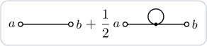

Without DeclareCoupling[lambda] the weight would be −λ/2. For one picture only, the option "Couplings" -> {lambda} does the same as the declaration.

More

• An interaction declared in another style (DeclareInteractionLine[W, "DoubleWavy"]) still stands for minus itself; a line declared only with DeclareLineStyle (a phonon, "Dashed") is a propagator and stands for itself. The option "Interactions" -> {W} treats W as an interaction line in one picture.
• An anomalous line ("DivergingArrows", "ConvergingArrows") shows no orientation: the weight reads it along its fermion line, around a loop in either sense, along an open line from its end at the first external label.
• The manual, section The weights, has the details; Conventions the signs of the propagators.