Goal of the Program

The goal of this program is to solve the time dependent Schrodinger equation. Notice this is different than the time independent version which is an eigenvalue problem. Let's work in 2 dimensions where our independent variables are $x$ and $t$. Thus our equation becomes:

$iℏ \frac{\partial }{\partial t}Ψ(x,t)$ = $[\frac{-ℏ^2}{2m} \frac{\partial ^2}{\partial x^2} + V(x)]Ψ(x,t)$

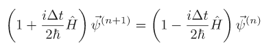
We will use the Crank Nicholson method. Writing everything in terms of operators, we can see the right hand side is really just the hamiltonian operator so now we have

$\frac{\partial}{\partial t}Ψ(x,t) = \frac{-i}{\hbar}\hat{H}Ψ(x,t)$

The next step here is to discretize $Ψ(x,t)$ as a vector: $Ψ(x,t_n)$ -> $\vec{ψ^n}$ where $Ψ(x_j,t_n) = \vec{ψ_j^n}$. We then discretize the Hamiltonian as a matrix, The Crank-Nicolson method is to split up the Hamiltonian, half explicit and half implicit: $\frac{\partial}{\partial{t}}Ψ(x,t) = \frac{\vec{ψ^{n+1}} - \vec{ψ^n}}{Δt}$ = $\frac{-i}{\hbar}\hat{H}Ψ(x,t) = \frac{1}{2}(\frac{-i}{\hbar}\hat{H}\vec{ψ^{n+1}} - \frac{i}{\hbar}\hat{H}\vec{ψ^n})$

or

$(1 + \frac{i\Delta t}{2\hbar}\hat{H})\vec{ψ^{n+1}} = (1 - \frac{i\Delta t}{2\hbar}\hat{H})\vec{ψ^n}$

where $1$ is the identity matrix and \hat{H} is our discretized hamiltonian matrix. When we solve for $\vec{ψ^{n+1}}$ we get

$\vec{ψ^{n+1}}$ = $(1 + \frac{i\Delta t}{2\hbar}\hat{H})^{-1}(1 - \frac{i\Delta t}{2\hbar}\hat{H})\vec{ψ^n}$

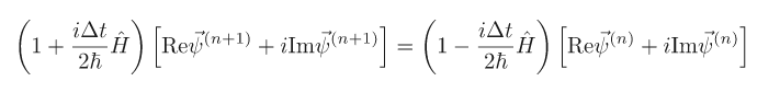
As you can see, this problem requires complex variables. One can either code the problem using complex variables, or recast it as a purely real problem. The linear algebra subroutines I wrote are for real numbers only so I will instead make it a purely real problem. We can rewrite

as

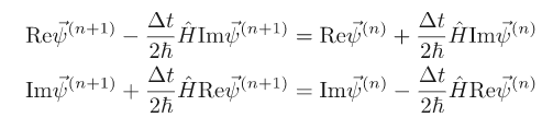
This results in 2 coupled equations:

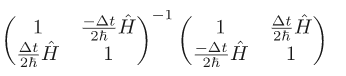
We can write these as block matrices or a "super matrix" if you will. It is a mathematical object that looks like a 2x2 matrix but each element itself is a matrix. So we have:

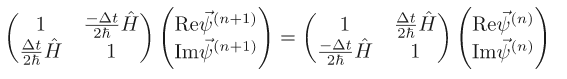
Therefore if the wave function is discretized as a (complex) vector of length , we replace it with a purely real vector of length $N$ and purely real matrices of size $2N$ x $2N$. To evolve from time $t_n$ to time $t_{n+1}$ start with the $2N$ sized vector

and perform the matrix multiplication:

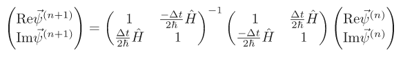
Since the matrices on the right hand side of the equation contain only constants you can store the result of multiplying the second one by the inverse of the first one and use it to evolve for as many time steps as necessary.

The probability densities are then given by:

$p(x_j, t_n) = |Ψ(x_j,t_n)|^2 = Re(\psi_j^n)^2 + (Im \psi_j^n)^2$

Part I

We will put the wavefunction in a box from $ -L to L$ and set $V(x) = 0$. We implicitly have a boundary condition that the wavefunction vanishes at the boundaries. We set $\hbar = m = 1$. Let's have the initial wave function be a gaussian: $Ψ(x,t = 0) = (2\pi\sigma^2)^{-1/4}exp(\frac{-(x-x_0)^2}{4\sigma^2})$. The input for these parameters will be received via namelist:

The size of the box : length

The number of sample points in : n_points

The number of time steps: n_steps

The size of the time step : delta_t

The width of the Gaussian wave function : width

The center of the Gaussian wave function : center

The oscillator parameter : k_oscillator (For the next part)

A file name for the results as a function of time: time_file

A file name for the results of the probability density: density_file

After reading the input parameters the program will sample the lattice points. This will allow us to set the initial wave function to the Gaussian expressed above. Then the code will construct the time evolution matrix:

Remember that the wave function will be an array of size 2n_points. The first half contains a sampling of the real part of $\vec{\psi^n}$ , while the second half contains a sampling of the imaginary part. For the initial Gaussian (which is purely real) the second half will be all zeros. In the same vein, the time evolution matrix will be a 2n_points by 2*n_points matrix.

Then we can evolve you wave function and store the different snapshots in the time_wave_function array. Then we can calculate the following expectation values for every time step.

Normalization: $\Sigma_j p_j dx$ which is constant

Expectation value of position: $(x) = \Sigma_j x_j p_j dx/\Sigma_i p_i dx$

Width: $\sigma = \sqrt{(x^2) - (x)^2}$ where $(x^2)$ = $\Sigma_j x^2_j p_j dx/\Sigma_i p_i dx$

Finally into two different files you will find the results. One file should contain those expectation values (one per column) as a function of time. The second file should contain a few snapshots of the probability density at different times.

The time evolution of the width can actually be computed analytically as: $\sigma(t) = \sqrt{\sigma^2_0 + \frac{\hbar^4 t^2}{4m^2\sigma_0^2}}$

where is the initial width from the namelist file.

We can confirm that the width grows, initially, according to the analytic prescription. After some time it will deviate because of the wall. We can see this in jupyter.

Part II

Now let's throw the wavefunction into a harmonic oscillator where $V(x) = \frac{1}{2}kx^2$. Now we want to follow $(x)$ as a function of $t$. Classically we should expect $(x(t)) = x_0cos(sqrt{\frac{k}{m}t}$. We can compare it to what we get numerically in jupyter.

Compiling

It would be quite beneficial to you if you had a Linux system because it would enable you to use the makefile included.

If this is the case then what you do is open a terminal, use the cd command to change to this directory.

Then type make.

You'll see some gfortran commands being executed. All of this has created an exectuable file called schrodinger.

In order to run this executable you type ./schrodinger This will make the program compile with default values which produce results of the part of the project with V(x) and k equal to 0. However if you want to run with the harmonic oscillator then do ./schrodinger parameters.namelist which sets k = 1.0.

You can edit the namelist input yourself to see how the output changes, slight deviations in initial conditions can wildly change the graph of the probability densities!

Next you can type jupyter notebook into the terminal to see the graphs of the probability densities and expectation values.