Home
The aim of the project is to make the reservoir computing methods easy to use and available for .net platform without dependency on external heterogeneous libraries. Two main reservoir computing methods are called Echo State Network (ESN) and Liquid State Machine (LSM). The implemented solution supports both of these methods. However, since ESN and LSM are based on very similar principles, RCNet brings the option to combine them at the same time. This approach, as I believe, opens up new interesting possibilities. This general implementation is called "State Machine" in the context of RCNet.
I have no ambition to describe here the principles of the reservoir computing paradigm theoretically, there are many available documents on the Internet that explain the issue in detail. Primary aim of these pages is to describe the use of the RCNet library and I want to keep things as simple as possible. Still, I will allow a very brief introduction to the reservoir computing concept to facilitate understanding of RCNet library purpose.
Recurrent neural networks (RNNs) are very well suited for processing time-dependent data such as
- Forecasting the development of time series
- Classification (pattern recognition, etc.)
Reservoir computing makes it possible to use the benefits of the recurrent network very efficiently. Efficiency lies in the fact that the synapses and their weights in the recurrent network (called reservoir) are randomly chosen at the beginning and remain fixed (in contrast with traditional training methods for RNNs). Only the Readout layer is trained, most often very simply, by the linear regression.

- The input data is inserted into the reservoir via special input neurons (yellow balls). The task of input neuron is only to mediate external input and facilitate its delivery into the reservoir through synapses.
- Recurrently connected hidden neurons (blue balls) do the nonlinear transformation and provides reservoir dynamics. Input signal of each hidden neuron consists of summed weighted output signals from connected hidden neurons and input neurons. This can be a little confusing. Everyone probably thinks of the order in which the hidden neurons count their signals? The answer is simple. It does not matter. The signal that provides the neuron to other neurons corresponds to the state at the last completed recomputation of the entire reservoir (T - 1).
- At each time point, the historical and current input data are described by the current state of the reservoir neurons. The states of reservoir neurons are so-called predictors (In fact, the relationship of the current state of the neuron to the predictor is a bit more complicated and it will be explained later in detail)
- Predictors are sent to be processed by the readout layer
- The reservoir is simply the data preprocessor
- The reservoir typically contains hundreds (and sometimes thousands) of recurrently connected neurons
- The influence of historical data on the current states of hidden neurons is weakening in time. The memory capacity of the reservoir depends on several aspects, such as the number of hidden neurons, the type and setting of hidden neurons, the density of the interconnection and the type of used synapses
- The weights of the synapses play an important role. It is necessary to ensure that the input signal will pass through the reservoir and pass through it without the neurons being oversaturated.
- The rich reservoir dynamics allows to train readout layer to map the same predictors to the different outputs (predictions) at the same time
- Different uses require different reservoir handling. There is a big difference between the continuous predictions of time series and classifications. For the time series, it is necessary to ensure that the states of the neurons are not affected by the initial state of the reservoir. This is solved by the fact that the first N reservoir states are not sent as the predictors to the readout layer (aka Reservoir boot phase). It is also necessary to keep the current neuron states for the next prediction when new input data (T + 1 time) is available. In the case of a classifier, it is different. Here is an input pattern (sequence) that represents time-dependent data and a decision is expected. In this case, it is the mistake to keep states of the reservoir neurons from the previous pattern/decisions. The reservoir starts for each pattern from the beginning. The entire pattern is processed by the reservoir and only the final state of the neurons is sent as the predictors to be processed on readout layer
Simplified training scenario:
- Collect all known input and desired output data
- Normalize and standardize the data
- Through reservoir, transform the collection of input data into a collection of predictors
- Train readout layer to be able to map the predictors to the desired outputs
The use of a trained network:
- Get next known input data
- Normalize and standardize the data by the same way as during the training
- Through reservoir, transform the input data into the predictors
- Push predictors into the readout layer and let it to compute outputs (predictions)
Hidden neuron and its Activation function
In general, neuron is a small computing unit that processes the input signal (stimulation) and produces an output signal. The way neuron processes the input signal to output signal defines its so-called Activation Function. The neuron can be simply understood as the envelope of its activation function, where the neuron provides the necessary interface and the activation function performs the core calculations. Activation functions (and therefore also neurons) are distinguished into two types: Analog and Spiking. For a better insight into the activation functions, look at the wiki pages.
Analog activation function has no similarity to behavior of the biological neuron. It is always stateless, which means that the output value (signal) does not depend on the previous inputs but only on current input at the time T and particular transformation equation (usually non-linear).
A typical example of the analog activation function is TanH (hyperbolic tangent), which non-linearly transforms the input value to the output in the range (-1, 1)

Spiking activation function attempts to simulate the behavior of a biological neuron that accumulates (integrates) input stimuli on its membrane potential and when the critical threshold is exceeded, fires a short pulse (spike), returns the membrane to its initial state and the cycle starts from the beginning. In other words, the function implements one of the so-called Integrate and Fire neuron models. For a better insight into the biological neuron models, look at the wiki pages.
It is obvious that spiking activation function is time-dependent and must remember its previous state.
The following figure illustrates the progress of membrane potential under constant stimulation. The figure is from the great online book Neuronal Dynamics and shows the behavior of the "Adaptive Exponential Integrate and Fire" model (class AdExpIF in RCNet).
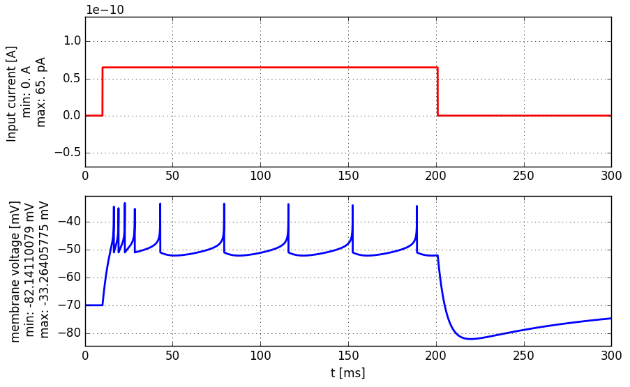
Note that the membrane potential (blue line) is not an output signal. The output signal consists of nine short constant pulses (spikes) at time points where membrane potential exceeds the firing threshold -40 mV. So the output is a zero signal and only at firing times the signal has a value of 1.
Input neuron has associated no activation function and is very simple. Its purpose is only to mediate external input and facilitate its delivery into the reservoir's hidden neurons through synapses.
The readout layer task is to map predictors from the reservoir to the values of one or more network output fields. The so-called supervised training is used and each output field is trained separately. The most commonly used technique is linear regression where weights (linear coefficients) are searched that best directly map the predictors to the corresponding desired output field values.