About

Included here are some code snippets from my project.

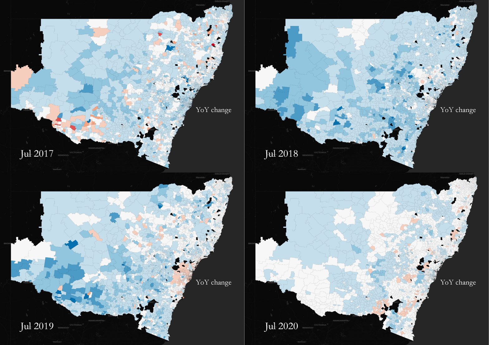
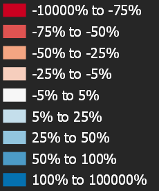
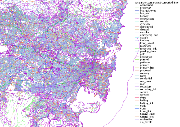
YoY land value percentage change across NSW, Australia. Some suburbs change in tandem, some are outliers.

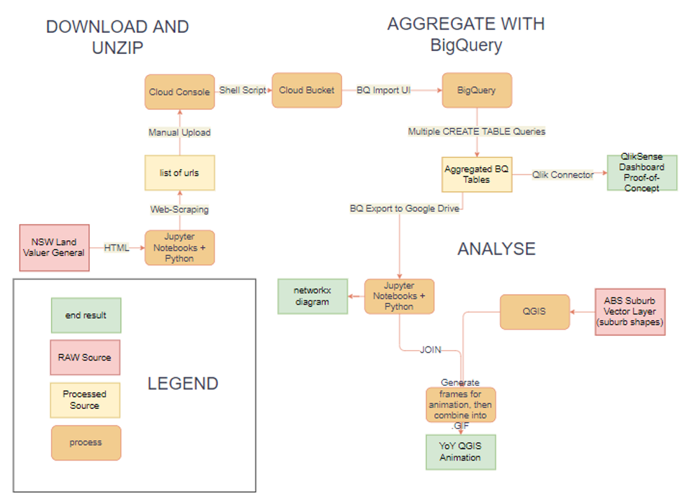
The data pipeline to get the data from it's raw source state into the various visualisations.

for filepath in $(ls ~/land-value-data/*.zip)
do
	echo "Processing ${filepath}"
	if unzip $filepath -d ~/land-value-data/ ; then
		echo "${filepath} unzip success!"
		if gsutil -m cp ~/land-value-data/*.csv gs://super-bucket-man/land-value-data ; then
			echo "CSVs copied successfully! Deleting files."
            rm -f ~/land-value-data/*.csv
			rm -f $filepath
		else
			echo "CSVs copy failed.
		fi
	else
		echo "unzip failed. try again for file: ${filepath}"
	fi
	
	echo "remaining files:"
	ls ~/land-value-data/*.zip
done

The shell script used to unzip and transfer the raw data from the cloud shell to the cloud bucket. It extracts and deletes each .ZIP file sequentially in order to stay under the cloud shell's 5GB storage limit.

CREATE OR REPLACE TABLE `showcase-presentation.fullscale_dataset.suburb_aggregated_data` AS (
    SELECT
        ld.SUBURB_NAME, 
        lv.DATE_MONTH, 
        AVG(lv.LAND_VALUE) as avg_land_value,
        COUNT(ld.PROPERTY_ID) as property_count
    FROM 
        `showcase-presentation.fullscale_dataset.land_data_raw` AS ld
    INNER JOIN
        `showcase-presentation.fullscale_dataset.land_values` AS lv
        ON lv.PROPERTY_ID = ld.PROPERTY_ID
    GROUP BY
        ld.SUBURB_NAME, lv.DATE_MONTH
    ORDER BY 
        avg_land_value DESC, 
        lv.DATE_MONTH ASC, 
        ld.SUBURB_NAME DESC
);

BigQuery query is then exported, processed in a Jupyter Notebook, then the result is used as the data source for the map above.

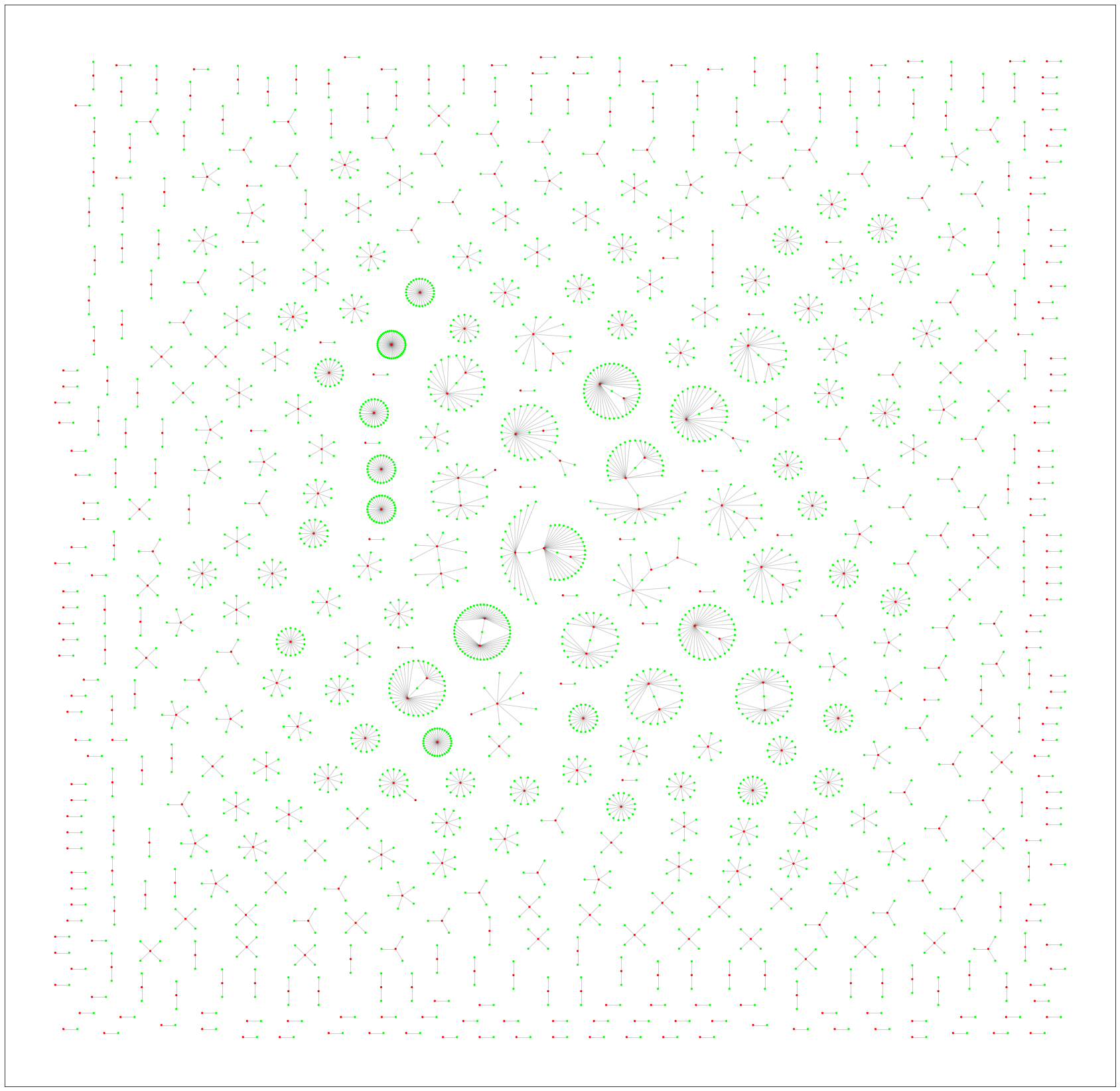
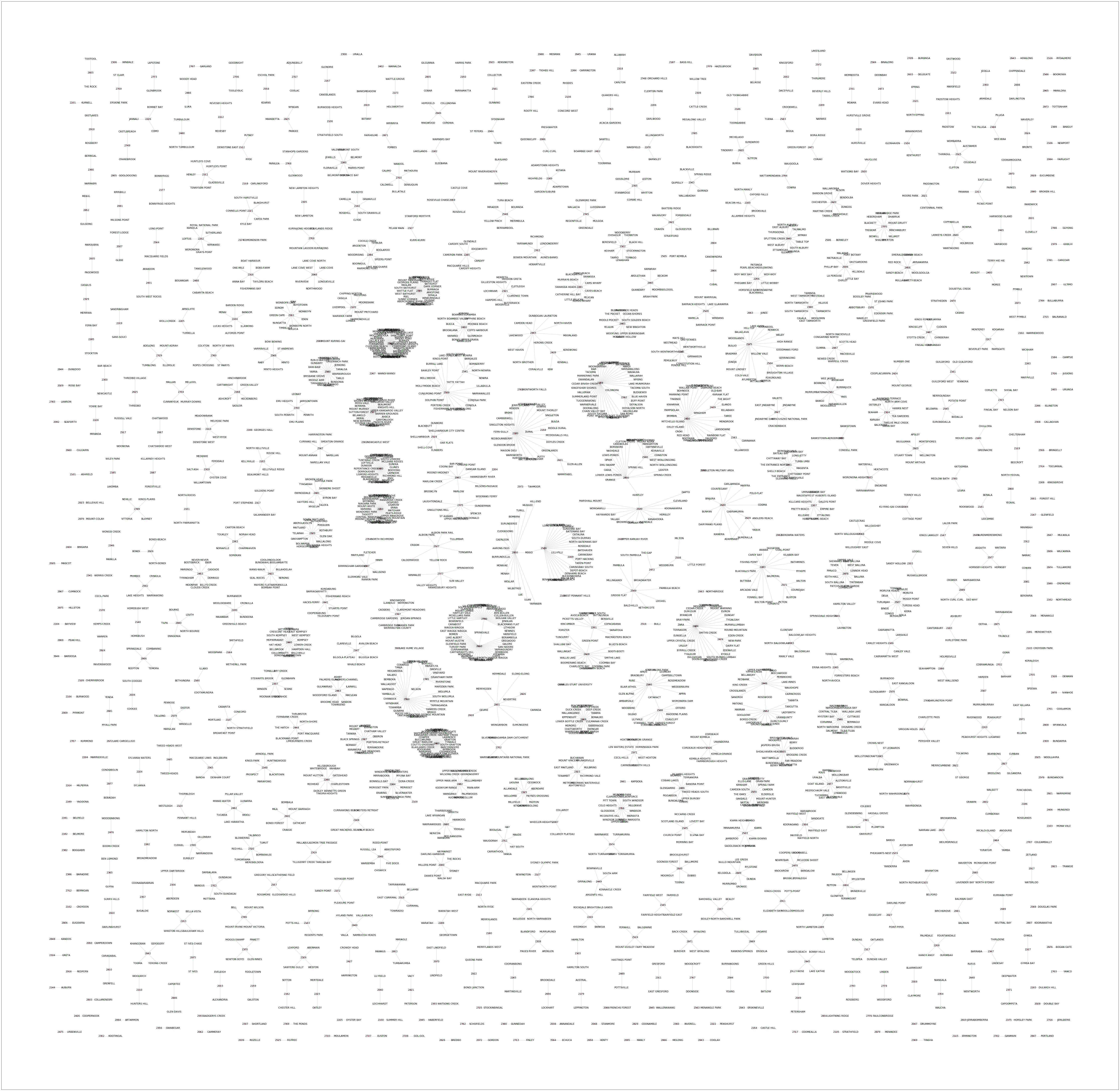
networkx diagram showing a subset of the unique pairs of suburb_name, postcode. It demonstrates that there's actually a m:n relationship going on.

Same as above, but with labels.

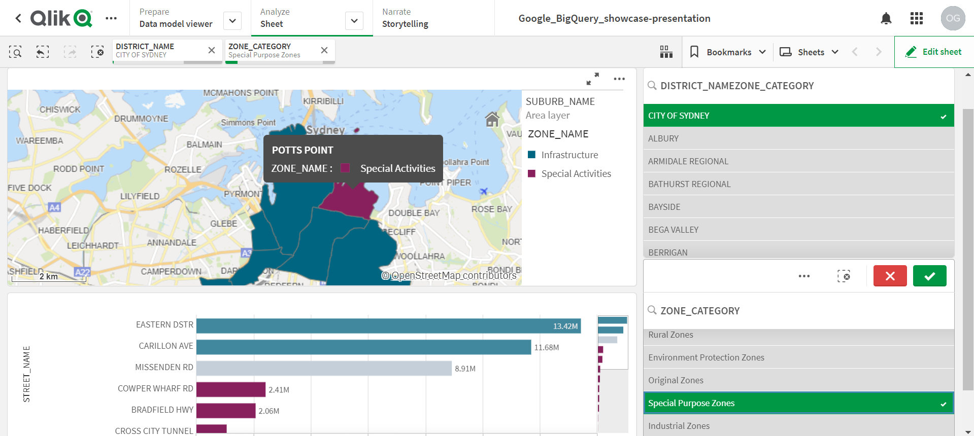
QlikSense Dashboard proof of concept

CREATE OR REPLACE TABLE `showcase-presentation.fullscale_dataset.street_name_agg_table` AS (
    SELECT
    -- inefficient way of retrieving the higher level granularities for the STREET_NAME
        MIN(ld.DISTRICT_NAME) AS DISTRICT_NAME, 
        MIN(ld.SUBURB_NAME) AS SUBURB_NAME, 
        MIN(ld.POSTCODE) AS POSTCODE, 
        ld.STREET_NAME, 
        -- gets first element from an array of structs, 
        --   then gets the string value corresponding to the "value" key
        APPROX_TOP_COUNT(ld.ZONE_CODE, 1)[OFFSET(0)].value AS most_frequent_zone_code,
        AVG(lv.LAND_VALUE) AS avg_land_value,
        AVG(ld.AREA_M2) AS avg_area_m2
    FROM 
        `showcase-presentation.fullscale_dataset.land_details_latest` AS ld
    INNER JOIN 
        `showcase-presentation.fullscale_dataset.land_values` AS lv ON lv.PROPERTY_ID = ld.PROPERTY_ID
    WHERE 
        ld.STREET_NAME IS NOT NULL
    GROUP BY 
        ld.STREET_NAME
    ORDER BY
        avg_land_value DESC
) 

BigQuery Query used to make the above QlikSense PoC

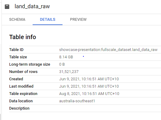
Before I realised that the source was duplicating data, the 12 .zip files uncompressed + BQ denormalisation created this crazy 8.14GB table.

OSM Street data

PROs and CONs of BigQuery

PROs

• no keys
  • my data had duplicate property IDs.
• RECORD datatypes: ARRAYs and STRUCTs
  • interesting way to denormalise data whereas regular SQL would have been incapable
• easy to setup databases
  • schema gets inferred. In my case this was desirable
• first TB of queries is free
• data is stored internally by column, so queries will only process the columns that are necessary for the query versus the whole table

CONs

• append only
  • as such it is suboptimal for data cleaning
• couldn't automatically delete a tmp table / view
• can't import from a zip file containing .csv files
  • this is why I needed to unzip in the Cloud Shell