CompChem Tools
Whilst there are number of Open Source computational toolkits and command-line tools they often present a step learning curve for new users. In an effort to provide a simpler environment to access these tools this page will highlight a series of Jupyter notebooks that users can use to run key computational studies that might be undertaken in a drug discovery project.
To use these notebooks you will need to have Jupyter and a number of Python libraries installed. The easiest way to do this is to use Anaconda. Anaconda is a modern package manager and seems to be becoming the preferred source of scientific software.
Everyone is welcome to contribute Jupyter notebooks, I'd certainly recommend reading "Ten simple rules for writing and sharing computational analyses in Jupyter Notebook" DOI which gives some great tips.
Whether you use notebooks to track preliminary analyses, to present polished results to collaborators, as finely tuned pipelines for recurring analyses, or for all of the above, following this advice will help you write and share analyses that are easier to read, run, and explore.
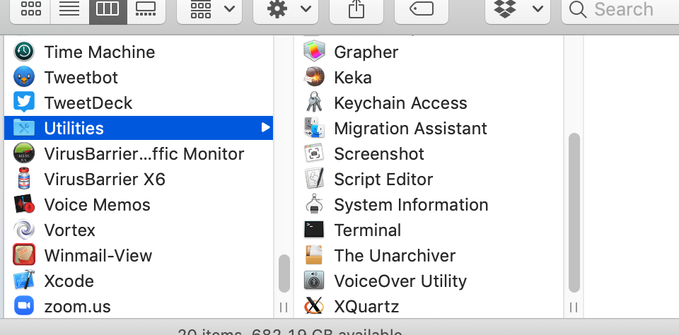
To run these tools you will need a little familiarity with using the command-line interface. On a Mac this is the Terminal app found in the Utilities folder in the Applications folder. If you want a quick introduction to the UNIX command line try Learn UNIX in 10 minutes
Install Conda using the instructions here https://www.anaconda.com/distribution/
Then in a terminal window type
conda install jupyter
conda install -c rdkit rdkit
conda install numpy
conda install scipy
conda install scikit-learn
conda install pandas
conda install matplotlib
conda install seaborn
You should now have all the components installed to run Jupyter notebook. To run a notebook you need to use the Terminal to navigate to the folder containing the notebook, use the unix command cd (change directory) followed by the path to the folder.
cd /Users/username/Projects/OpenSourceAntibiotics/UsingSmina
If you then type ls (List) you should a listing of all files within the folder.
ls
373ligand_only.pdb			protein_minus_ligand.pdb
ConformationGenerationDocking.ipynb	protein_plus_373ligand.pdb
asinexSelection.sdf
To start the Jupyter kernel in the Terminal type
Jupyter notebook
You should see the jupyter server start up in the Terminal and your web browser open showing the list of files in the folder.
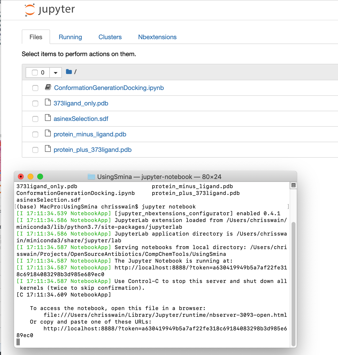
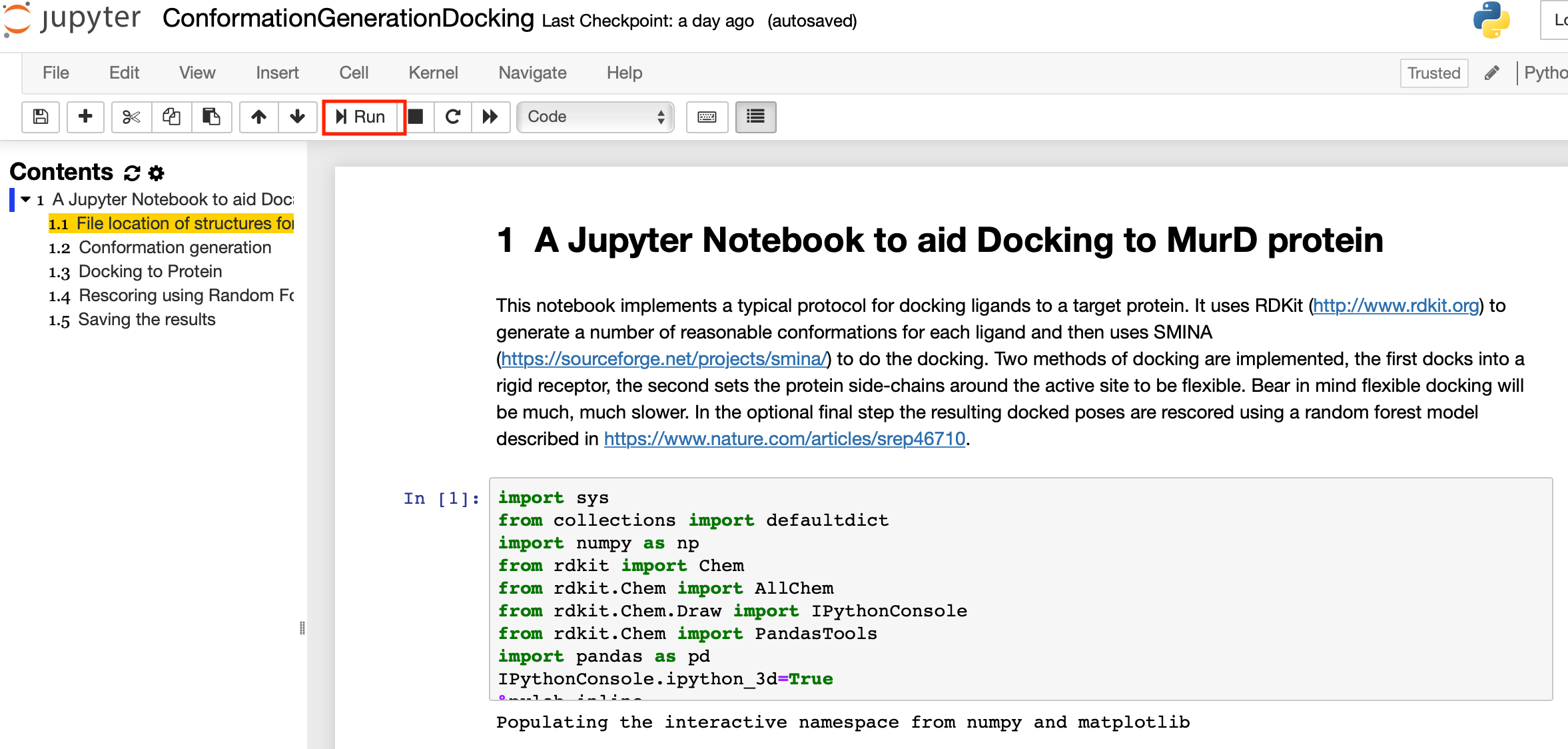
Now click on the link ConformationGenerationDocking.ipynb
This will open the notebook, you should now be able to step through the cells in the notebook by clicking the run arrow in the notebook menu bar.
SMINA (https://sourceforge.net/projects/smina/) is a command-line application for docking. Instructions for installation are on the website. By default it will be installed in
/usr/local/bin/smina.osx
After you have installed smina you need to give it permission to execute using the Terminal command
chmod +x /usr/local/bin/smina.osx
You can then check it is all working by typing in the Terminal
/usr/local/bin/smina.osx --help
and you should see the Smina help.
DataWarrior is a free application for visualisation, filtering and analysis of chemical datasets. Most of DataWarrior's functionality is described in detail in its user manual. DataWarrior installers for Linux, Macintosh and Windows can be downloaded from the download page. There is a demo workflow here that gives you an idea how you might go about selecting/filtering a compound dataset prior to running a docking exercise.
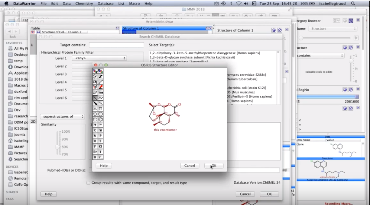
There is a video describing it's use here https://youtu.be/ReaPf9xmTR8
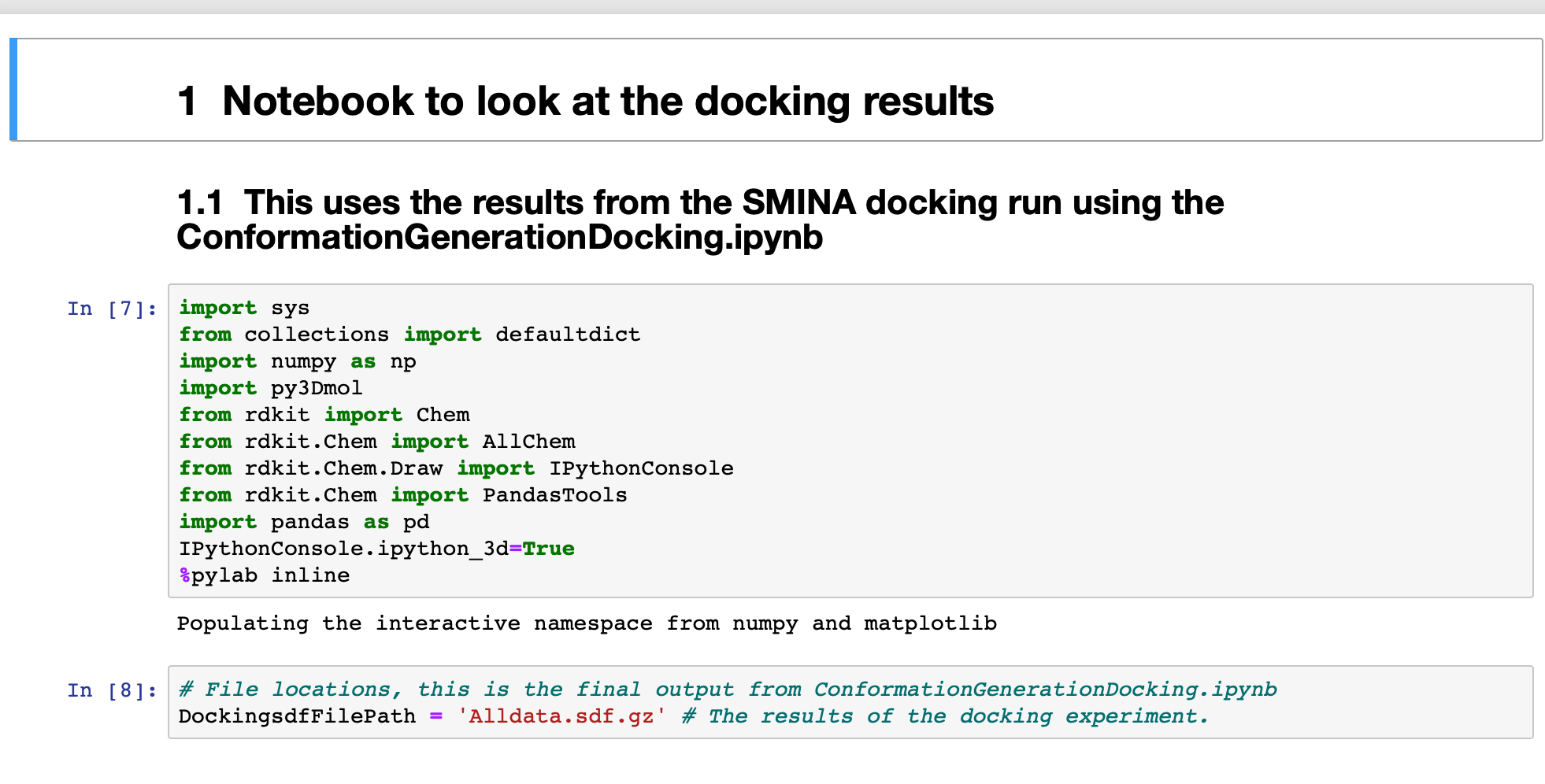
This notebook implements a typical protocol for docking ligands to a target protein. It uses RDKit (http://www.rdkit.org) to generate a number of reasonable conformations for each ligand and then uses SMINA (https://sourceforge.net/projects/smina/) to do the docking. Two methods of docking are implemented, the first docks into a rigid receptor, the second sets the protein side-chains around the active site to be flexible. Bear in mind flexible docking will be much, much slower. In the optional final step the resulting docked poses are rescored using a random forest model described in this publication DOI. You can read more details of the notebook here and you can download a folder containing the notebook and the necessary files here.
Having run the docking experiment the next task is to select molecules for purchase/testing, while you could simply select the top 10% scoring structures it is always worth having a look at the docked structures to see if any have bad conformations or contain reactive functional groups. This notebook aims to help with the sorting and selecting.
To do this we need a couple of other tools these can be installed by typing the following commands into the Terminal.
pip install py3Dmol
conda install openbabel
conda install -c schrodinger pymol
py3Dmol allows display of 3D structures in the Jupyter notebook, openbabel is a cheminformatics library and pymol is a molecular viewer for both biomolecules and small molecules.
The notebook uses the result of the Docking/Scoring notebook (Alldata.sdf.gz) as input and the protein that was used for the docking (protein_minus_ligand.pdb). As it is written it assumes these two files are in the same folder as the notebook.
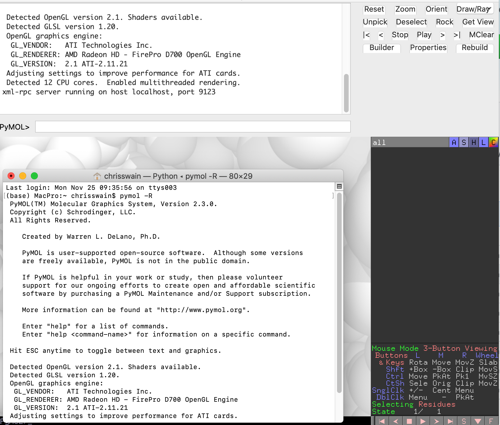
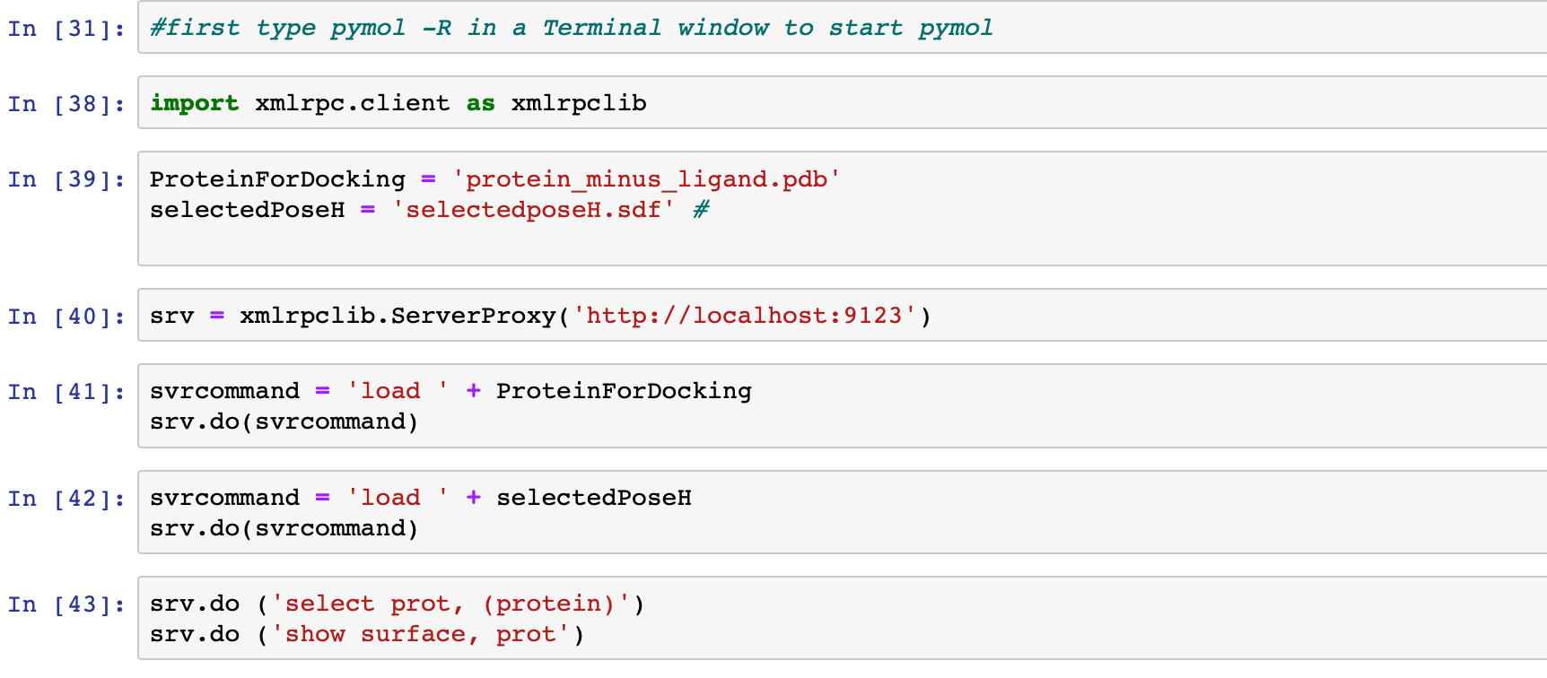
A key feature of this notebook is the use of Pymol as the external molecule viewer, we need to start it in manner that will allow remote commands. In the Terminal type
pymol -R
The start up text should include
xml-rpc server running on host localhost, port 9123
We can now send commands to Pymol using this port.
You can read more about the notebook here and download the notebook and the necessary files here.
Key section on sending commands to Pymol is shown below, the full list of available command is here.
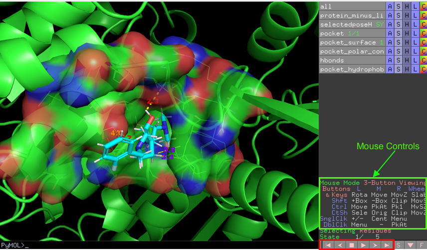
If you have selected more than one molecule from the docking you should be able to browse through them using the buttons highlighted in red in the bottom write corner of the Pymol window.
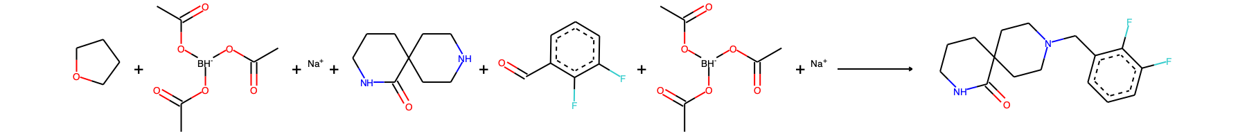
IBM RXN is a free web service for predicting reactions and retrosynthesis described in this publication.
Similar to other work, we treat reaction prediction as a machine translation problem between SMILES strings of reactants-reagents and the products. We show that a multi-head attention Molecular Trans-former model outperforms all algorithms in the literature, achieving a top-1 accuracy above 90% on a common benchmark dataset. Our algorithm requires no handcrafted rules, and accurately predicts subtle chemical transformations. Crucially, our model can accurately estimate its own uncertainty, with an uncertainty score that is 89% ac-curate in terms of classifying whether a prediction is correct. Furthermore, we show that the model is able to handle inputs without reactant-reagent split and including stereochemistry, which makes our method universally applicable
It can be accessed via a web interface at https://rxn.res.ibm.com/rxn/sign-in and it also has a documented API which was updated recently. A python wrapper for the IBM RXN api has been published and it was available on GitHub. https://github.com/rxn4chemistry/rxn4chemistry
To install use PIP
pip install rxn4chemistry
You then need to register and get an api key here https://rxn.res.ibm.com/rxn/user/profile.
The website gives instructions on how to access the various api elements, the following Jupyter notebook uses the retrosynthesis option.
The first part of the script imports a set of selected structures from a docking run and displays the structures in a Pandas data frame.
selected_df = PandasTools.LoadSDF(SelectedsdfFilePath,molColName='Molecule', removeHs=True)
We then add a SMILES string we will use to send to the web service.
selected_df['SMILES'] = selected_df.Molecule.apply(Chem.MolToSmiles)
You can then choose the molecule you want to make, and submit the SMILES for retrosynthesis suggestions.
response = rxn4chemistry_wrapper.predict_automatic_retrosynthesis(product=theSMILES)
# rerun this until the status is 'SUCCESS', keep in mind the server allows only 5 requests per minute
# and a timeout between consecutive requests of 2 seconds
#If it times out, wait a couple of minutes and rerun.
import time
while True: results = rxn4chemistry_wrapper.get_predict_automatic_retrosynthesis_results(response['prediction_id']) if results['status'] == 'SUCCESS': break time.sleep(30) #check every 30 secs
There are limits to how often you can poll the server so we need to include a delay. Once it has completed we can get the results
You can read more details of the notebook here
This notebook demonstrates how to get the structures and data from the master worksheet, then convert the SMILES to molecule objects using RDKit that allow some simple manipulations and visualisations. SMILES (Simplified Molecular Input Line Entry System) is a line notation (a typographical method using printable characters) for entering and representing molecules and reactions. https://www.daylight.com/dayhtml/doc/theory/theory.smiles.html You can read more details of the notebook here and you can download the notebook here.