Related individuals

Related individuals

SUMMIT's h² and rg estimators assume an unrelated GWAS sample. Close relatives share untagged genetic variation and often environment, so including them inflates the estimates. Pruning to an unrelated set avoids this but discards people, which matters most in small or admixed cohorts.

This workflow keeps every individual and removes the related pairs from the estimating equations instead. Run the GWAS on everyone as usual. SUMMIT then computes the related pairs' part of each trait's association statistics, REL_M, from the genotypes and phenotypes. By default this is one number per trait, which is added to the summary statistics as a constant column and subtracted by summit --h2. The estimate stays unbiased whatever the phenotypic covariance between relatives. Methods gives the estimating equations.

For a runnable synthetic example of the whole workflow (sibling pairs, h² and rg), run bash example/related_individuals.sh from the repository root.

Inputs

• The BED genotypes used for the GWAS. summit relatives moments does not yet read PGEN.
• A phenotype table with FID IID followed by one or more phenotype columns, as given to the GWAS.
• The GWAS covariates, FID IID followed by numeric columns, without an intercept column. Use exactly the covariates of the GWAS, including genotype PCs.
• A pair table with IID1 IID2, optionally FID1 FID2 and a kinship column.
• GWAS summary statistics from ordinary least squares on all individuals with those covariates, for example PLINK 2 --glm. Mixed-model statistics (BOLT-LMM, REGENIE, fastGWA) are not valid inputs.

IID1 IID2 RELATEDNESS
SIM000001 SIM000002 0.51
SIM000002 SIM000417 0.06

Listed pairs are closed into families (connected components) by default, and every within-family pair is excluded. --no-closure excludes only the listed pairs. With --kinship-col and --kinship-min, only pairs above the threshold in that column are used. For relatedness (twice the kinship coefficient), 0.0442 keeps fourth-degree and closer relatives and is a reasonable default.

SUMMIT's PC-adjusted GRM on LD-pruned SNPs and PC-Relate give practically the same families. KING-robust overstates kinship for individuals of intermediate ancestry and should not define pairs in recently admixed cohorts. Compute PCs on unrelated individuals and project relatives onto them (PC-AiR) so that families do not form their own components.

Compute related-pair moments

summit relatives moments \
  --geno study.bed --pheno phenotypes.tsv --covar covariates.tsv \
  --pairs pairs.tsv --kinship-col RELATEDNESS --kinship-min 0.0442 \
  --out results/relmoments

The command writes:

• results/relmoments.rel_m.tsv: one row per phenotype, PHENO N N_COVARIATES PAIRS REL_M, where REL_M is the related-pair moment per SNP in HE scale (the V-weighted mean over SNPs of the per-SNP moments). With --annot annot.txt, a partitioning annotation such as SUMMIT's MAF/LD bins, the table also has one REL_M_<class> column per class, for partitioned fits.
• results/relmoments.json and results/relmoments.log.

One genotype pass gives the values of every phenotype. Each phenotype keeps its own complete-case sample, related pairs, covariate projection and N_eff, as in a GWAS that drops missing values, and its values equal those computed from the per-SNP moments of that sample. Missing genotypes are mean-imputed, which agrees with complete-case GWAS to first order in the missing fraction. The pass reads all genotypes but forms the projected genotypes only for people in families, so its cost is mainly reading the genotypes, plus the number of related pairs times the number of SNPs. REL_M does not depend on allele coding.

One value per trait keeps the point estimate of the single-component model, and of each class of the annotation used, exactly as with per-SNP values when the LD scores come from the same sample (with LD scores from another sample, the two differ only through the difference between the samples' V weights). Only the jackknife changes, because each block's share of the total is then proportional to its number of SNPs (weighted by V). In UK Biobank simulations this moved standard errors by less than 0.1% (Simulations).

--per-snp also writes the exact per-SNP values, results/relmoments.tsv.gz (CHR SNP BP A1 A2 and one REL_M_<phenotype> column per phenotype). This needs one genotype pass per distinct complete-case sample, and append and cross-m12 accept the file in place of the per-phenotype tables.

Add --cross to write results/relmoments.rel_m12.tsv, the cross-trait value REL_M12 for every pair of phenotypes (see Genetic correlation). With --per-snp it covers only pairs with the same complete-case sample. When the LD scores are computed in the study itself, the LD-score step adds the relatives' share (see LD scores).

Estimate h²

Add the column to the summary statistics and fit as usual:

summit relatives append --sumstats trait.sumstats.gz \
  --rel results/relmoments.rel_m.tsv --pheno TRAIT --out trait.rel.sumstats.gz

summit --h2 trait.rel.sumstats.gz --ldscores reference.gw.ldscore.gz \
  --out results/trait

append writes the trait's value in a REL_M column, the same for every SNP. For a partitioned fit, run moments and append with the same --annot, and each SNP gets its class's value. When a summary-statistics file has a REL_M column, SUMMIT subtracts it from each SNP's HE-scale moment. Annotations, partitioned models and every jackknife design work unchanged. The log reports c_rel and the number of distinct REL_M values; SNPs with a missing REL_M are dropped. --h2-batch-fast does not accept REL_M.

A study that releases summary statistics can add the constant REL_M column itself, as it adds COV_RANK. Users then fit them with the related pairs excluded and need nothing else, unless they compute LD scores in the same sample.

Inbreeding (optional)

Each individual is also paired with themselves in the h² estimating equation, with the weight K_ii, the diagonal of the GRM. Inbred individuals have a larger K_ii. When their residual variance is also larger, for example because the effects of untagged causal variants grow with inbreeding, the fit credits that excess to the SNPs. This happens in related and unrelated samples alike. Add --inbreeding to moments to leave these diagonal terms out of the equation as well, in the same way as the related pairs:

summit relatives moments --geno study --pheno phenotypes.txt --covar covariates.txt \
  --pairs pairs.tsv --kinship-col RELATEDNESS --kinship-min 0.0442 --inbreeding \
  --out results/relmoments

Nothing else changes. append copies three more values (REL_S, REL_LAMBDA and REL_DIAG, plus one REL_DIAG_<class> column per class with --annot), and summit --h2 uses them whenever they are present. The log then says "diagonal terms left out of the estimating equations". REL_S depends on the phenotype; REL_LAMBDA and REL_DIAG depend only on the genotypes, the covariates and the related pairs. The option also removes the small bias from the related pairs' leverage on the covariates.

With LD scores computed exactly in the GWAS sample, the estimate equals the individual-level method-of-moments estimate whose first equation uses only pairs of different, unrelated individuals (tested to a relative difference of 1e-7). The cost is precision, because the diagonal terms also carry a little information. In exact calculations for UK Biobank cohorts of 4,000 to 9,000 people (South Asian and African ancestry, 10 to 20 PCs), the standard deviation of the estimate was 2% to 3% larger, and in a European cohort of 15,000 less than 0.1% larger. The bias it removed in these cohorts was a few percent of the standard error, about the same as this cost. The cost falls with sample size, so the option is most useful in large samples with much inbreeding. The extra genotype pass projects the genotypes of everyone in each complete-case sample, which adds roughly one GWAS-sized projection per sample. For genetic correlation, run moments with --cross --inbreeding; cross-m12 then also writes REL_S12, the cross-trait value, and summit --rg leaves the diagonal terms out of both h² fits and the cross-trait equations. This needs the values in both summary-statistics files and in the --rel-m12 file, and the overlapping covariance in HE scale (--pheno-rg/--pheno-rg-cov or --overlap-covariance-rg) rather than an estimated intercept, with the jackknife or delta standard errors; SUMMIT stops with a message if any of these is missing. --per-snp works with --inbreeding too: the run's PREFIX.rel_m.tsv and PREFIX.rel_m12.tsv hold the values, and append and cross-m12 read them next to the per-SNP table. LDSC weighting (--weight-mode ldsc) runs on LD scores without the V column, whereas these values are defined with it, so it refuses them. A mean shift with inbreeding (inbreeding depression) is handled by adding an inbreeding coefficient to the covariates of the GWAS, moments and the LD scores.

The --inbreeding values are one number per phenotype (and class), which gives exact point estimates but leaves the deleted block's diagonal terms in every jackknife replicate. In UK Biobank cohorts the jackknife SE was within 1% of the exact replicate-wise SE with 8 MAF-LD bins and 200 blocks, and within 4% with chromosomes, and it erred on the conservative side.

Long-range LD correction of standard errors

The block jackknife sees the covariance of the moments within each block but not the covariance between blocks. In admixed and other structured samples that covariance comes from long-range LD and from the self-pair terms, whose K_ii tracks ancestry on every chromosome, so the jackknife SE is too small. --long-range-se adds it back. It needs the share of the LD-score mass that comes from SNP pairs in different blocks, which summit relatives longrange computes from the GWAS genotypes:

summit relatives longrange --geno study --covar covariates.txt --pairs pairs.tsv \
  --kinship-col RELATEDNESS --kinship-min 0.0442 --annot mafld8.annot --out results/longrange
summit --h2 study.with_rel_m.tsv --ldscores study.gw.ldscore.gz --annot mafld8.annot \
  --long-range-se results/longrange --out results/h2

The variance is then

Var = V_jk / (1 - rho_s - rho_l (1 + 2 h2)) + 4 h2^2 (1 - sum f^2) / n

rho_s is the part of the between-block share carried by the self-pair terms and rho_l the rest, which comes from long-range LD. Long-range LD also links the blocks' genetic-signal terms, hence the factor 1 + 2 h2. The second term is the variance of products of different blocks' genetic values, which the jackknife misses even in homogeneous samples; f are the blocks' shares of the SNPs and n is the sample size. Fits with the moments --inbreeding values have no self-pair part. Negative shares are set to 0, so the corrected SE is never below the jackknife SE.

longrange writes bin-by-bin sums, with and without self-pairs, for the chromosome design and for 200 blocks (--nblocks), so one file serves --njack 200 and --njack chr. Run it on the GWAS samples with the GWAS covariates and the fit's annotation. The results table then has h2_se (corrected), h2_se_jk, jk_factor and long_range_rho. The pass holds the projected genotypes in memory (4 bytes per sample and SNP). With 8 MAF-LD bins and 100 probes it took 1.5 to 6.5 minutes on 16 cores for 3,400 to 12,000 people and 0.4 to 1 million SNPs.

In UK Biobank cohorts the corrected SE was 0.98 to 1.02 times the exact rescaled SE with 8 MAF-LD bins, and 1.00 to 1.19 times with one component, against 0.89 to 1.00 for the jackknife alone. At h² of 0.25 and 200 blocks the correction raised the SE by about 1% in white British participants, 5% to 11% in South Asian participants, 5% to 7% in African-European admixed participants and 5% in a wider African-ancestry group.

--rg takes the same option. Each trait's h² SE is corrected as above. For the genetic covariance, 1 + 2 h2 becomes

m12 = (w1 + 2 w2 + 3 w3) / (w1 + w2 + w3)

with w1 = (1 - h1)(1 - h2) + (c - g)^2, w2 = h1 (1 - h2) + h2 (1 - h1) + 2 g (c - g) and w3 = h1 h2 + g^2, where g is the genetic covariance and c the overlapping covariance in HE scale, and the second term becomes 2 w3 (1 - sum f^2) / n. The ratio of the corrected to the jackknife variance of the genetic covariance is applied to rg. Only the totals change; per-bin SEs are the jackknife SEs, and the log lists the jackknife SEs of the totals. In the same cohorts the rg SE was 0.99 to 1.03 times the exact rescaled SE with 8 MAF-LD bins.

--jk-traces, with the traces of summit relatives traces, computes the exact rescaling SE_jk * sqrt(AV / E[V_jk]) from the traces of every pair of blocks. The traces are much larger and tied to the SNP set; use them to check the correction.

LD scores

LD scores	Use when	Extra step
A matched reference, or the study's unrelated subset	The LD-score sample has the ancestry composition of the full GWAS sample	None
In-sample, on all GWAS individuals	Admixed or structured cohorts	Subtract the relatives' share

In recently admixed cohorts, an unrelated subset chosen by kinship pruning can have a different ancestry composition from the full cohort, and therefore different admixture LD. Its LD scores then misstate the trace for the full sample. In a UK Biobank admixed cohort this lowered h² by about 9%; in-sample LD scores removed the bias.

In-sample LD scores include the relatives' pairs. Give the LD-score step the same pairs and options as moments:

summit --geno study.bed --covar covariates.tsv \
  --relative-pairs pairs.tsv --kinship-col RELATEDNESS --kinship-min 0.0442 \
  --nvecs 20000 --block-size 16384 --num-threads 16 --out ld/study

ld/study.gw.ldscore.gz then has one LD_REL_<column> column per LD-score column, holding the related pairs' share of that LD score. Fit with this file as usual. --h2 and --rg subtract LD_REL for summary statistics with REL_M and use the LD scores unchanged otherwise; the log says which. The LD-score step uses every sample with complete covariates, regardless of phenotype missingness, and computes LD_REL with the same samples, covariates, annotation and V weights as the LD scores. Partitioned LD scores need no extra option, whatever the annotation. --relative-pairs reads BED or PGEN and applies to genome-wide LD scores only.

An LD-score file without LD_REL columns is taken to come from unrelated individuals.

Genetic correlation

Pair exclusion must cover both h² denominators and the cross-trait moment:

summit relatives moments --geno study.bed --pheno phenotypes.tsv \
  --covar covariates.tsv --pairs pairs.tsv --cross --out results/relmoments
summit relatives append --sumstats a.sumstats.gz --rel results/relmoments.rel_m.tsv \
  --pheno A --out a.rel.sumstats.gz
summit relatives append --sumstats b.sumstats.gz --rel results/relmoments.rel_m.tsv \
  --pheno B --out b.rel.sumstats.gz
summit relatives cross-m12 --rel results/relmoments.rel_m12.tsv \
  --pheno1 A --pheno2 B --out a_b.relm12.tsv

summit --rg a.rel.sumstats.gz,b.rel.sumstats.gz --rel-m12 a_b.relm12.tsv \
  --ldscores reference.gw.ldscore.gz \
  --pheno-rg a.pheno.tsv,b.pheno.tsv --pheno-rg-cov covariates.tsv,covariates.tsv \
  --out results/a.b

a_b.relm12.tsv holds the pair's single REL_M12 value. For a partitioned fit, give cross-m12 the annotation used in moments (--annot): the file then holds each SNP's class value. --rel-m12 also accepts the value itself, or a per-SNP file from --per-snp --cross. SUMMIT requires REL_M in both files and --rel-m12. With only some of them, the pairs would be removed from some estimating equations and kept in others. With in-sample LD scores that carry LD_REL, the same file serves h² and rg. Two phenotypes measured in different complete-case samples are each projected and normalized in their own sample, as in their GWAS. REL_M12 then sums over related pairs with one member in each sample, and its weights are sqrt(V_a V_b). The same genotype pass computes it for every pair of phenotypes. Its cost grows with the square of the number of phenotypes times the number of related pairs: in the EUR cohort below (40 phenotypes in 33 complete-case samples, 4,216 pairs) the pass took 35 minutes on 16 cores. For these pairs --inbreeding writes no REL_S12. The sample-overlap covariance describes each person's own two phenotypes and needs no change.

In rg manifest mode, give each pair's --rel-m12 file or value in an optional rel_m12 column. --long-range-se applies to every pair, and the results table then also has the jackknife SEs (rg_total_se_jk and the others), jk_factor_rg and long_range_rho. --rg-manifest-fast accepts neither REL_M nor these options.

Simulations

We simulated phenotypes from UK Biobank genotypes in three cohorts that include relatives, with families defined by GRM relatedness above 0.0442.

Cohort	Individuals	Maximal unrelated subset	Within-family pairs	SNPs	PCs
EUR	14,561	12,151	4,216	454,207	10
SAS	8,566	7,484	2,506	448,403	20
AFR	4,327	3,903	721	1,002,034	10

Every SNP had an effect, except in scenario E, where 1% of SNPs did. The heritability was 0.25, or 0.10 in scenario D. In scenarios B to E, relatives also shared an untagged genetic component with variance 0.25 and covariance proportional to their relatedness. In scenarios C to E they also shared a household effect with variance 0.10. Scenario A had neither. Each scenario had 100 replicates. The GWAS used PLINK 2 with the PCs as covariates, and the summary statistics carried COV_RANK. Each analysis used in-sample LD scores with the V column, computed in its own GWAS sample, and 200-block jackknife standard errors. We compared the maximal unrelated subset with everyone, keeping or excluding the related pairs. The truth is the simulated heritability.

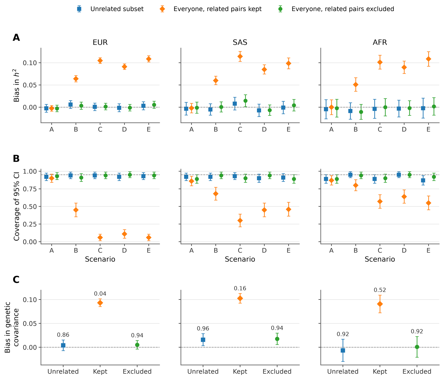
Excluding related pairs gave unbiased estimates in every cohort and scenario (panel A), and so did the unrelated subset. Keeping the related pairs biased h² upward by 0.05 to 0.11 whenever relatives shared more than the SNP kernel. Confidence intervals from excluding pairs covered the truth in 89% to 95% of replicates (panel B). Coverage was lowest in the admixed AFR cohort, where jackknife standard errors are somewhat small.

For genetic correlation we simulated 50 pairs of traits per cohort with h² 0.25 and rg 0.5, in which relatives also shared correlated untagged and household effects. The overlap covariance came from --pheno-rg and --pheno-rg-cov, and the pair-excluded fits used REL_M in both files and --rel-m12. Excluding related pairs estimated the genetic covariance as well as the unrelated subset did, and keeping them inflated it by 0.09 to 0.10 (panel C; labels give the coverage of 95% intervals).

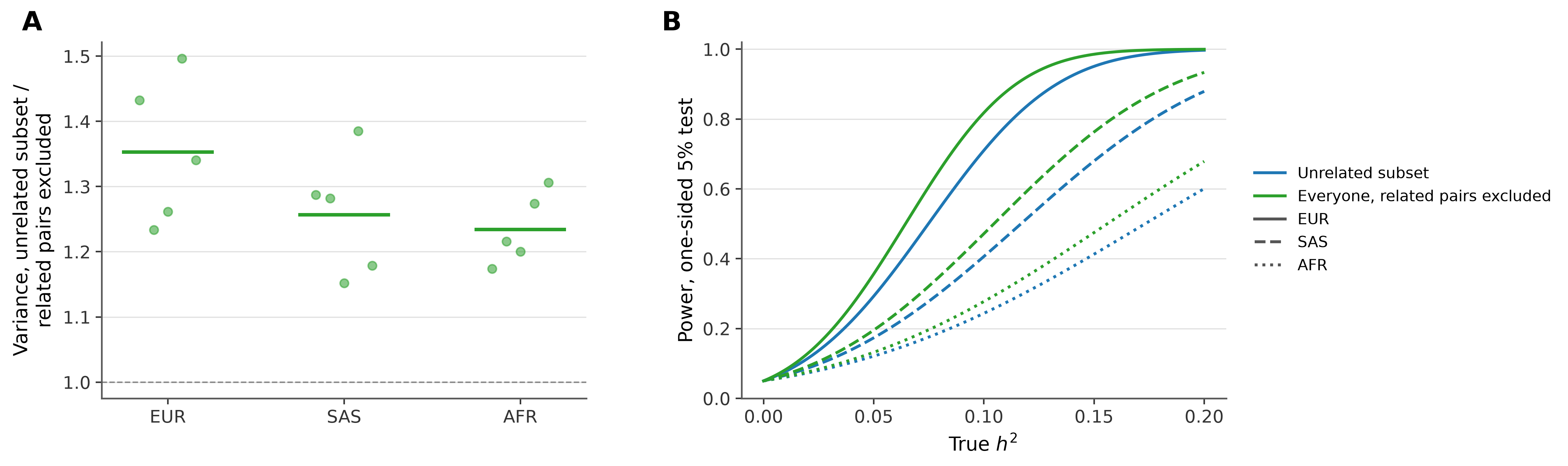
Keeping everyone made the estimates more precise. The sampling variance of the unrelated-subset estimate was 1.15 to 1.50 times that of the pair-excluded estimate (panel A), a mean of 1.35 in EUR, 1.26 in SAS and 1.23 in AFR, where 17%, 13% and 10% of individuals were outside the unrelated subset. Panel B shows the power to detect heritability at the 5% level implied by each analysis's sampling variance.

The simulations used per-SNP REL_M. Refitting every pair-excluded analysis with one value per trait (the default) left the h² and rg estimates unchanged. It moved the jackknife standard errors by +0.01% to +0.09% on average (0.993 to 1.009 times the per-SNP standard error in individual fits) and left coverage unchanged in every cohort and scenario. The genetic-covariance standard errors moved by +0.08% to +0.10%. A second approximation, which spread each total in proportion to a genotype-only per-SNP sum over the related pairs, did no better.

In AFR, the same pair-excluded analysis with ordinary LD scores (--snp-var-weights-off) underestimated h² by 0.010 to 0.023 because the PCs explain part of the genotype variance (LD scores).

The simulation and plotting scripts are in benchmarks/related_individuals/.

Interpretation

The estimate is the SNP heritability of the SNPs in the GRM, the quantity SUMMIT estimates in unrelated samples. Covariance between relatives from shared environment or untagged variants is removed with their pairs, whatever its form. Pairs below the threshold remain; their contribution scales with their squared relatedness and is small for distant relatives.

Jackknife standard errors are computed as for unrelated samples. With one REL_M value per trait, a deleted block removes the related pairs' part in proportion to its SNPs rather than its own part; the simulations below compare both.

A single REL_M value per trait is a weighted sum of phenotype products over all related pairs and reveals little about any one pair. Per-SNP values computed from few pairs carry information about those individuals' genotypes and phenotypes. Keep --per-snp output in the secure environment where it was computed. Binary traits (PCGC) are not covered.