Problem modelling soil water with Richards Equation

[dfalster]

knitr::opts_chunk$set(echo = TRUE)

knitr::opts_chunk$set(echo = TRUE)
library(tidyverse)
library(deSolve)
library(patchwork)
library(ggplot2)

Background and Aims

This report aims to implement and document soil water models in R, so that we can better better understand challenges we've had implementing this in the C++ model.

We encountered the issue that soil water model was running very slowly and erratically. Initially, we thought this might be due to some programming errors. However, it appears that it may be the equations themselves.

DF ran some checks, working off a branch in plant with only the soil water layer added, i.e no consumption of water by plants: becb153

Richards equation

I first investigated the possibility of programming errors. What i found was that it works fine if you set the rate of change in theta so a constant or a variable value, dpeending on depth and/or time (e.g. $\sin(t)/z$, to make it interesting. Also it was very quick (as expected, e.g. with 100 soil layers for 300 years -> 1.84 sec), and the ODE system seems to be sized correctly. This is as expected and so suggests memory allocation etc is all fine.

speed

Note, We can get RE to run with time step of 1e-6.
Other models talk about using a 30min timestep. In years, 30min = 5.7e-5 (=1/(242365)), so not that different!
But a single RK step is actually 4 smaller steps,

Original multi-layer model based on Richards Equation.

To clarify issues with the model I implemented the same equations in R using deSolve package.

# Model parameters
params <- c(soil_moist_sat = 0.453, 
            K_sat  = 440.628, 
            soil_moist_sat = 0.453, 
            n_psi = 4.8,
            a_psi = 8.7,
            b_infil = 8.0,
            rain = 1,
            n = n
            )

# Equations - ported from C++ version
pow <- function(x,y){x^y}

soil_K_from_soil_theta <- function(theta, K_sat  = 440.628, soil_moist_sat = 0.453, n_psi = 4.8) {
  K_sat * pow(theta/soil_moist_sat, 2*n_psi + 3)
}

psi_from_soil_moist <- function(soil_moist, soil_moist_sat = 0.453, a_psi = 8.7, n_psi = 4.8) {
  a_psi * pow(soil_moist/soil_moist_sat, -n_psi)
}

rates <- function(t, theta, params) {
  with(as.list(c(theta, params)), {
    
    psi <- psi_from_soil_moist(theta, soil_moist_sat = soil_moist_sat)
    K <- soil_K_from_soil_theta(theta, soil_moist_sat = soil_moist_sat)
    
    q <- rep(NA_real_, n+1)
    dz <- rep(2/n, n)
    dtheta_dt <- rep(NA_real_, n)
    
    # Calculate fluxes at boundaries
    # top boundary layer - depends on soil water content
    q[1] = rain *
        # fraction of precipitation infiltrating
        max(0.0, 1 - pow(theta[1] / soil_moist_sat, b_infil))
    
    # Boundary below each node, except the last one
    # Eq. 3 + 11, Ireson et al. (2023)
    for (i in seq_len(n-1)) {
      dpsi_dz = (psi[i + 1] - psi[i]) / dz[i]
      q[i + 1] = 0.5 * (K[i] + K[i + 1]) * (dpsi_dz - 1)
    }

    # lower boundary - free drainage boundary, Eq. 13 from Ireson et al. (2023)
    q[n+1] = K[n]

    # Set change in soil water content for each node
    for (i in seq_len(n)) {
      # Eq. 10, derivative of flux at node w.r.t to depth
      dq_dz = (q[i + 1] - q[i]) / dz[i]
      
      # Eq. 2, but we have subtracted resource depletion rates
      dtheta_dt[i] = -dq_dz
    }

    return(list(dtheta_dt))
  })
}

# Solve 
solve <- function(times, rates, state, method = "rk4", output = "theta") {
  ode(
    y = state,
    times = times,
    func = rates,
    parms = params,
    method = method) %>% 
  as_tibble() %>% 
  pivot_longer(-time, names_to = "depth", values_to = output)
}

plot_solution <- function(solution) {
  solution %>% 
  ggplot(aes(y = theta, x = time, col=as.character(depth))) +
  geom_line() +
  theme_minimal()
}

What we found was that the equations showed exactly the same pathologies as in the C++ version.

• It crashes when the step size becomes larger, e.g. > 1e-5 yr (which is ~5mins, 1e-536524*60))
• Works ok when step size is smaller

Works with small step size, 1e-5

n <-10
params$n <- n
# intiial state
state <- rep(0.2533, n)
# check rates function works
rates(0.1, state, params)

solution <- solve(times = seq(0,1, by = 1e-5), rates=rates, state=state, method="rk4")
plot_solution(solution)

Fails with larger step sizes, > 1e-5

solution <- solve(times = seq(0,1e-3, by = 1e-4), rates=rates, state=state, method="rk4")
plot_solution(solution)

Below are plots i captured in different runs. This was interesting, because we used the same timestpes as in plant and it failed at exactly the same spot

jpg")

It's a stiff system! Works when switching to different solver

However, changing the ode solving method fixes things (in the R version). Using lsoda instead of rk4 enables me to step with steps sizes of 0.1 out to 1 or more years.

solution <- solve(times = seq(0,1, by = 0.1), rates=rates, state=state, 
                  method="lsoda")
plot_solution(solution)

It seems this set of equations is stiff! According to wikipedia:

• Stiff equation:"a stiff equation is a differential equation for which certain numerical methods for solving the equation are numerically unstable, unless the step size is taken to be extremely small. It has proven difficult to formulate a precise definition of stiffness, but the main idea is that the equation includes some terms that can lead to rapid variation in the solution. When integrating a differential equation numerically, one would expect the requisite step size to be relatively small in a region where the solution curve displays much variation and to be relatively large where the solution curve straightens out to approach a line with slope nearly zero"
• Runge Kutta: "Explicit Runge–Kutta methods are generally unsuitable for the solution of stiff equations because their region of absolute stability is small; in particular, it is bounded. This issue is especially important in the solution of partial differential equations..... The advantage of implicit Runge–Kutta methods over explicit ones is their greater stability, especially when applied to stiff equations."
• Explicit_and_implicit_methods: "Implicit methods require an extra computation, and they can be much harder to implement. Implicit methods are used because many problems arising in practice are stiff, for which the use of an explicit method requires impractically small time steps $\Delta t$ to keep the error in the result bounded"

It also works fine if we enforce a consistenly short

solution <- solve(times = seq(0,1e-2, by = 1e-5), rates=rates, state=state, 
                  method="rk4")
plot_solution(solution)

Looking back at the literature this seems to make sense

• the literature on solving Richards equations is large, several people note issues with numerical stability
• Several papers talk about the complexity of siolving the equations
  • Fartjing 2017 Numerical Solution of Richards' Equation: A Review of Advances and Challenges: https://acsess.onlinelibrary.wiley.com/doi/full/10.2136/sssaj2017.02.0058
  • Bonan 2019 <>
• Ian Harmman mentioned that the SLI version of CABLE (Haverd and Cuntz 2010, 10.1016/j.jhydrol.2010.05.029), uses an adaptive time step, explicit method – but it has been shown to require very small time steps in some circumstances to ensure stability.
• The paper by Ireson 2024 recommending using Adaptive time solvers, does mention LS-ODA and calculating the Jacobian, both of which are typical for methods handling stiff systems.

Richards' equation is a nonlinear, degenerate, parabolic-elliptic partial differential equation (PDE). The elliptic nature of the solution can arise when capillary head is the primary variable, which is common in simulations of layered soils because capillary head is the continuous variable while water content is discontinuous across layers [List and Radu, 2016]. Numerical solvers for parabolic PDEs are not appropriate for elliptic PDEs.

Ogden et al 2017:

"The Richards equation is called a “degenerate” PDE because the strongly nonlinear coefficients in the equation approach zero in parts of the solution domain. For instance, the soil capillary pressure approaches zero as the soil approaches saturation and the unsaturated hydraulic conductivity approaches zero as the soil dries. This latter property leads to the existence of wetting fronts in which moisture content values propagate with finite speed, in contrast to the behavior of solutions to linear analogs such as the heat equation [Barenblatt, 1952; Swartzendruber, 1969; Aronson, 1986; Vasquez, 2007]. Furthermore, the properties of the PDE change from parabolic to elliptic as the soil becomes saturated. Nonlinearities and the degeneracy make the design and analysis of numerical schemes to solve Richards' equation very difficult"

Farthing & Ogden 2017: Richards’ equation is a nonlinear, degenerate elliptic- parabolic partial differential equation (List and Radu, 2016). The head-based forms of the equation, Eq. [3–5], transition from parabolic to elliptic as the solution domain nears saturation unless storage effects are included (Ss > 0), in which case Eq. [5] remains parabolic. The nonlinearity and transition of type in different portions of the problem domain make it very difficult to solve using traditional analytical techniques, and it is impossible to solve in closed form except for a small number of special cases (Miller et al., 1998). This difficulty is only exacerbated by the range of initial and boundary conditions encountered in practice as well as by the nature of common soil water constitutive relations that can lead to solutions with low regularity (Alt and Luckhaus, 1983). Specifically, the solution depends on two empirical, highly nonlinear soil water constitutive relations: the unsaturated hydraulic conductivity function K(θ) that can be constant or very near zero for non-positive values of the capillary head, and the capillary head function Psi(θ) that can take on arbitrary small values for relative saturations near 100%. These extremes lead to degeneracy in the solution of Richards’ equation

Of course, many approximate, empirical, or completely arbitrary methods have been developed over the years to simulate the flow of water through unsaturated soils because of the real or perceived difficulties posed by the numerical solution of Richards’ equation.

*Computational inefficiency and lack of robustness in Richards’ equation solvers used in practice most often manifest as poor linear and nonlinear solver convergence and/or poor performance of the time integrator. Our view is that a significant portion of this poor convergence and instability arises from under resolution in space of sharp fronts or other phenomena where highly nonlinear soil properties change drastically over neighboring elements or cells. *

Psi based form or RE

The implementation above is the mixed form, as it contains both $\psi$ and $theta$

The psi based form is recommended by Ireson et al

First we need a function for $K(\psi)$. Combining the functions for $K(\theta)$ and $\Psi(\theta)$ gives

$$K(\Psi) = K_{sat} (\Psi/a_{psi})^{-(2 + 3/n_{psi})}$$
and
$$C(\psi) = \frac{d\theta}{d\Psi}$$
(I think, need to check.)

Checking new functions are consistent with previous

theta_from_psi <- function(psi, soil_moist_sat = 0.453, a_psi = 8.7, n_psi = 4.8) {
  soil_moist_sat* (psi/a_psi)^(-1/n_psi)
}

soil_K_from_soil_psi <- function(psi, K_sat  = 440.628, a_psi = 8.7, n_psi = 4.8) {
  K_sat * pow(psi/a_psi, -(2 + 3/n_psi))
}

#dθ/dψ 
C <- function(psi, soil_moist_sat = 0.453, a_psi = 8.7, n_psi = 4.8) {
  soil_moist_sat* (a_psi)^(1/n_psi) * (-1/n_psi) *  (psi)^(-1/n_psi -1)
}

data <- 
  tibble(theta = seq(0, 0.5, length.out=20)) %>%
  mutate(
    psi = psi_from_soil_moist(theta),
    theta2 = theta_from_psi(psi),
    K1 = soil_K_from_soil_theta(theta),
    K2 = soil_K_from_soil_psi(psi))

ggplot(data, aes(psi, K1)) +
  geom_line() +
  geom_line(aes(y=K2), col="red", lty="dashed") +
  scale_x_log10() +
  scale_y_log10()

ggplot(data, aes(psi, theta)) +
  geom_line() +
  geom_line(aes(y=theta2), col="red", lty="dashed") +
  scale_x_log10() +
  scale_y_log10()

Looks good!

# Model parameters
n <- 10
params <- c(soil_moist_sat = 0.453, 
            K_sat  = 440.628, 
            soil_moist_sat = 0.453, 
            n_psi = 4.8,
            a_psi = 8.7,
            b_infil = 8.0,
            rain = 1,
            n = n
            )

# Equations - ported from C++ version
rates_psi <- function(t, psi, params) {
  with(as.list(c(psi, params)), {
    
    K <- soil_K_from_soil_psi(psi)
    
    q <- rep(NA_real_, n+1)
    dz <- rep(2/n, n)
    dpsi_dt <- rep(NA_real_, n)
    
    # Calculate fluxes at boundaries
    # top boundary layer - depends on soil water content
    q[1] = rain *
        # fraction of precipitation infiltrating
        max(0.0, 1 - pow(theta_from_psi(psi[1]) / soil_moist_sat, b_infil))
    
    # Boundary below each node, except the last one
    # Eq. 3 + 11, Ireson et al. (2023)
    for (i in seq_len(n-1)) {
      dpsi_dz = (psi[i + 1] - psi[i]) / dz[i]
      q[i + 1] = 0.5 * (K[i] + K[i + 1]) * (dpsi_dz - 1)
    }

    # lower boundary - free drainage boundary, Eq. 13 from Ireson et al. (2023)
    q[n+1] = K[n]

    # Set change in soil water content for each node
    for (i in seq_len(n)) {
      # Eq. 10, derivative of flux at node w.r.t to depth
      dq_dz = (q[i + 1] - q[i]) / dz[i]
      
      # Eq. 2, but we have subtracted resource depletion rates
      dpsi_dt[i] = - 1/C(psi[i]) * dq_dz
    }

    return(list(dpsi_dt))
  })
}

n <-10
params$n <- n
# intiial state
state <- rep(psi_from_soil_moist(0.2533), n)
# check rates function works
rates_psi(0.1, state, params)

plot_solution2 <- function(solution) {
  solution %>% 
  ggplot(aes(y = psi, x = time, col=as.character(depth))) +
  geom_line() +
  theme_minimal()
}

Same issue here, works with small time step or using lsoda solver

solution_psi <- 
  solve(times = seq(0,1e-2, by = 1e-5), rates=rates_psi, state=state, method="rk4", output = "psi") %>%
  mutate(theta = theta_from_psi(psi))

plot_solution(solution_psi)

but not with larger time steps

solution_psi <- 
  solve(times = seq(0,1e-2, by = 1e-3), rates=rates_psi, state=state, method="rk4", output = "psi") %>%
  mutate(theta = theta_from_psi(psi))

plot_solution(solution_psi)

So there's possibly no advantage in running the psi based model

Theta based model (incomplete)

We can also write a version of the RE fully based on $\theta$. According to Bonan 2019: "The moisture-based, or $\theta$-based, equation uses $\theta$ as the dependent variable with

$$\frac{\partial \theta}{\partial t} = \frac{\partial}{\partial z} \left[D(\theta) \frac{\partial \theta}{\partial z} \right] + \frac{\partial K}{\partial z}$$

in which $D(\theta) = K(\theta)/C(\psi)$ is referred to as the hydraulic diffusivity (m2 s–1). In this equation, the specific moisture capacity appears within the spatial derivative."

Below not finished. Needs review

rates <- function(t, theta, params) {
  with(as.list(c(theta, params)), {
    
    K <- soil_K_from_soil_theta(theta, soil_moist_sat = soil_moist_sat)
    
    dtheta_dt <- rep(NA_real_, n)

    dK_dz <- rep(NA_real_, n+1)
    dtheta_dz <- rep(NA_real_, n+1)
    f <- rep(NA_real_, n+1)
    dz <- rep(2/n, n)
    
    # Calculate fluxes at boundaries
    # top boundary layer - depends on soil water content
    q_top = rain *
        # fraction of precipitation infiltrating
        max(0.0, 1 - pow(theta[1] / soil_moist_sat, b_infil))
    
    D = soil_K_from_soil_theta(theta)/C(psi_from_soil_moist(theta))
    
    # Boundary below each node, except the last one
    # Eq. 3 + 11, Ireson et al. (2023)
    for (i in seq_len(n-1)) {
      dtheta_dz = (theta[i + 1] - theta[i]) / dz[i]
    }

    # lower boundary - free drainage boundary, Eq. 13 from Ireson et al. (2023)
    
    
    # Set change in soil water content for each node
    for (i in seq_len(n)) {
      # Eq. 10, derivative of flux at node w.r.t to depth
      dF_dz = (q[i + 1] - q[i]) / dz[i]
            dK_dz = (K[i + 1] - K[i]) / dz[i]
      f[i + 1] =0.5 * (D[i] + D[i + 1]) * (dtheta_dz)
      
      # Eq. 2, but we have subtracted resource depletion rates
      dtheta_dt[i] = -dq_dz
    }

    return(list(dtheta_dt))
  })
}

Time delay model

I considered an option for stabilising the system, which was to use the running mean of infiltration and drainage. This didn't help.

For future reference, a running mean can easily be tracked using a Delay differential equation: https://en.m.wikipedia.org/wiki/Delay_differential_equation#Reduction_to_ODE.

if you have variable $x$, then solve for running mean of x, $\bar{x}$, by adding an extra ODE to track $$y = \bar{x}/k$$, where $k$ is the decay rate (memory, higher values = shorter memory) and
$$\frac{dy}{dt} = x - k y$$
with initial condition
$$y = x/k.$$

# Model parameters
params_d <- c(params, k = 2)

rates <- function(t, state, params) {
  with(as.list(c(state, params)), {
    
    theta <- state[1:n]
    inflow_delay <- state[n+1]
    outflow_delay <- state[n+2]
      
    q <- rep(NA_real_, n+1)
    dz <- rep(2/n, n)
    dtheta_dt <- rep(NA_real_, n)

    psi <- psi_from_soil_moist(theta, soil_moist_sat = soil_moist_sat)
    K <- soil_K_from_soil_theta(theta, soil_moist_sat = soil_moist_sat)
    
    inflow <- rain *
        # fraction of precipitation infiltrating
        max(0.0, 1 - pow(theta[1] / soil_moist_sat, b_infil))
    
    # Calculate fluxes at boundaries
    # top boundary layer - depends on soil water content
     q[1] = inflow_delay*k 

    d_inflow_delay = inflow - k*inflow_delay

     
    # Boundary below each node, except the last one
    # Eq. 3 + 11, Ireson et al. (2023)
    for (i in seq_len(n-1)) {
      dpsi_dz = (psi[i + 1] - psi[i]) / dz[i]
      q[i + 1] = 0.5 * (K[i] + K[i + 1]) * (dpsi_dz - 1)
    }

    # lower boundary - free drainage boundary, Eq. 13 from Ireson et al. (2023)
    d_outflow_delay = K[n] - k*outflow_delay

    q[n+1] = k*outflow_delay

    # Set change in soil water content for each node
    for (i in seq_len(n)) {
      # Eq. 10, derivative of flux at node w.r.t to depth
      dq_dz = (q[i + 1] - q[i]) / dz[i]
      
      # Eq. 2, but we have subtracted resource depletion rates
      dtheta_dt[i] = -dq_dz
    }

    return(list(c(dtheta_dt, d_inflow_delay, d_outflow_delay)))
      })
}


state <- c(rep(0.2789496, 10), 1/as.numeric(params_d["k"]), soil_K_from_soil_theta(0.2789496)/as.numeric(params_d["k"]))
rates(10, state, params_d)

# Solve the equations
times <- c(seq(0,0.1, by = 1e-3))

s_solution <-
  ode(
    y = state,
    times = times,
    func = rates,
    parms = params_d,
    method = "lsoda") %>% 
  as_tibble()

out <- s_solution %>% 
  rename( inflow_delay = `11`) %>%
  rename( outflow_delay = `12`) %>%
  mutate(
    inflow_delay = inflow_delay*as.numeric(params_d["k"]),
    outflow_delay = outflow_delay*as.numeric(params_d["k"])
    ) %>%
  pivot_longer(-time, names_to = "depth", values_to = "theta") 

out %>%
  filter(!grepl("delay", depth)) %>%
  ggplot(aes(y = theta, x = time, col=as.character(depth))) +
#  geom_point() +
  geom_line() +
  theme_minimal()

out %>%
  filter(grepl("delay", depth)) %>%
  ggplot(aes(y = theta, x = time, col=as.character(depth))) +
#  geom_point() +
  geom_line() +
  theme_minimal()

Soil water code.zip

Possible ways forward

Need to find a solution that works with Runge Kutta ODE stepping

1. Use RE, but enforce short time step.
2. Try variants

• Soil Moisture Velocity Equation (Ogden 2015, Ogden 2017)
  • variation on RE to model packets of water
  • Converts RE to ODE, so easily compatible with solvers
• Ross 2003 simplifctaion
• Green Armpit model

3. Use simplified model

• Single layer model
• two layer model (He et al 2021)
• AWRA / WLD/ W3
• DAVE model variant

environemnts with strong wet-dry signal, we want to capture plants

[dfalster]

Overview of approaches

Source: Ranatunga K et al. (2008) Review of soil water models and their applications in Australia. Environmental Modelling & Software 23: 1182–1206. DOI: 10.1016/j.envsoft.2008.02.003

Types of models

Fig. 1. Schematic diagram for basic processes employed by each category of water balance models identified in review by Ranatunga K et al. (2008). RF, ET and RO refer to rainfall, evapotranspiration and runoff.

• includes list of models applied in Australia (as of 2008)

D’Odorico P& Porporato A (Eds.) (2006) Dryland ecohydrology. Dordrecht, The Netherlands: Springer. - Chapter 3

Table 1: A classification of soil moisture models on the basis of different approaches used in the representation of soil, evapotranspiration, vegetation canopies, infiltration, and precipitation.

On single bucket models

• "The main limitation of this model is due to the use of only one soil layer. This approach does not allow for a calculation of the time needed by water to infiltrate to relatively deep soil layers and could lead to unrealistic soil moisture estimates at subdaily time scales. However, the comparison with the results of a more complex model based on the integration of Richards equation (1931) has shown (Guswa et al. (2002)) that that the two models provide similar results at the daily time scale. This is particularly true when roots are assumed to be able to extract more water from wet portions of the root zone to compensate for the lower uptake from the drier parts of the soil column. In some cases the single-layer (“bucket”) model has been modified by adding multiple layers. A simplified multilayer model of the water balance uses equation (1) for each layer, considering as main moisture input to the lower layers the drainage from the overlying soil (Parton et al., 1998). Studies at relatively short (subdaily) time scales or in deep soils still require the numerical integration of Richards’ (1931) equation through the soil profile (see Chapter 2)."

Parton, W.L., M. Hartman, D., Ojima, and D. Schimel (1998). DAYCENT and its land surface submodel: description and testing, Global and Planetary Change, 19: 35-48.

Guswa AJ et al. (2002) Models of soil moisture dynamics in ecohydrology: A comparative study. Water Resources Research 38: 5-1-5–15. DOI: 10.1029/2001WR000826

• Compares Richards to bucket model
• finds reasonable corrpeosndnace in spoil water

Figure 7 Traces of root zone saturation over the growing season for the average climate realization. The thick line is the result from the bucket model; the thin solid line is the result from the Richards model with f = 0.1; the dashed line is the result from the Richards model with f = 0.8.

Transpiration is OK, but evidenly diverging a bit

Figure 8 Traces of daily transpiration over the growing season for the average climate realization. The thick line is the result from the bucket model; the thin solid line is the result from the Richards model with f = 0.1; the dashed line is the result from the Richards model with f = 0.8.

"Therefore the differences in the results can be attributed to the spatial variability in soil moisture and its effect on local losses due to evaporation and transpiration. The biggest differences in the predictions from the bucket and Richards models are in the relationship between evapotranspiration and average root zone saturation, the timing and intensity of transpiration, and the partitioning of uptake between evaporation and transpiration. Whether or not these differences are significant will depend on the objective of the modeling study."

eSsenatil parts

Key elements of what we want

1. Control total rainfall amount

• This limits total amount of resource, and thus LAI, height and biomass

2. Wet-dry periods

• Temporal variation in rain. Mianly inetersted in major wet-dry periods
• lag effects: soil water carried over from one hydrological year into a subsequent hydrological year (means current annual rainfall not good predictor of soil water) [Cleverly 2016]

3. Differences in Effective Rooting Depth giving access to different soil water

• Chitra-Tarak R et al. (2021) on effecticve rooting doeth in BCI
• D’Odorico P& Porporato A (2006), citing Guswa AJ et al. (2002) suggest single bucket model can track dyanmics of richars in average water amount perfectly ok. But Guswa AJ et al. (2002) shows divergences in tracking traspiration, because of diffeerences where plants access water

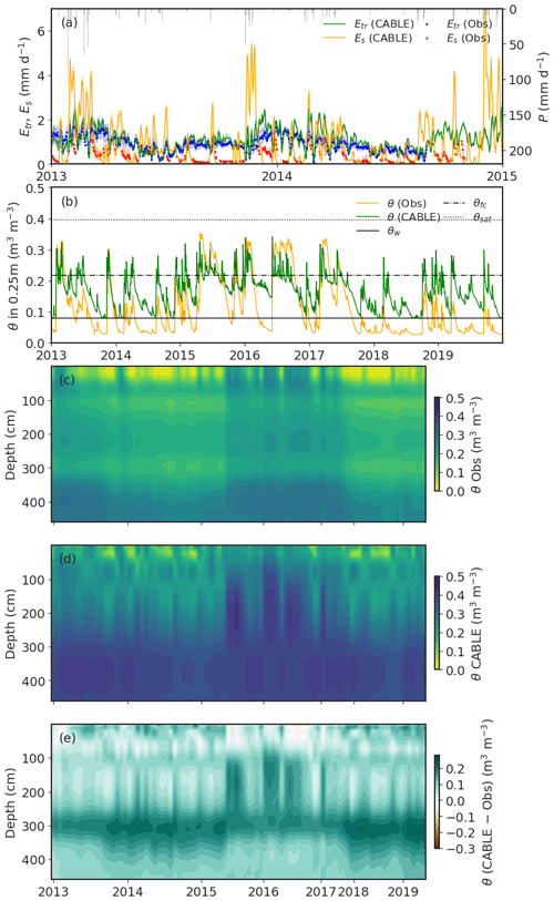
Glimpses at data

Data suggests water availability at deeper levels more stable.

Moist tropical forest

BCI, Chitra-Tarak R et al. (2021) Hydraulically-vulnerable trees survive on deep-water access during droughts in a tropical forest. New Phytologist 231: 1798–1813. DOI: 10.1111/nph.17464

BCI has a strong wet-dry season. Rainfall at BCI is seasonal with a mean annual total of 2627 mm and a pronounced dry season from mid-December through April with < 100 mm of rainfall per month.

Note top layer dries out much more.

EucFace Western Sydney

Mu M et al. (2021) Evaluating a land surface model at a water-limited site: implications for land surface contributions to droughts and heatwaves. Hydrology and Earth System Sciences 25: 447–471. DOI: 10.5194/hess-25-447-2021

• The site has a temperate–subtropical transitional climate with mean annual precipitation of 719.1 mm evenly distributed over the year.

Semi-arid woodland (Ti-trees basin)

Cleverly J et al. (2016) Soil moisture controls on phenology and productivity in a semi-arid critical zone. Science of The Total Environment 568: 1227–1237. DOI: 10.1016/j.scitotenv.2016.05.142

• The presence of a hardpan is an important feature of many semi-arid environments, having the potential for affecting local (i.e., fine scale) distributions of moisture availability ... Hardpans in the strongly weathered red earths (kandosols) of Australia can be deep (> 3 m to the top of the hardpan), but large areas of the continent exist over a shallow hardpan buried between 0.3 and 1 m below the surface (Morton et al., 2011). Because of this variation, siliceous hardpans could have a profound effect on local hydrology and θ. In landscapes containing a hardpan barrier to drainage, the total capacity for storage of water above the hardpan as soil moisture is proportional to the depth of unconsolidated soil above the hardpan. Thus, variability in hardpan depth is likely to affect plant and root distribution, which will then reinforce spatial patterns in θ. Consequently, Mulga density increases where depth to the top of the hardpan is large (Tongway and Ludwig, 1990), implying that Mulga density increases with soil moisture storage capacity above the hardpan.

• Located where soils have a large capacity for storage of water, and the storms to recharge θ are large and infrequent, Mulga is distributed in the more productive parts of the landscape (Murphy et al., 2010), where carbon is sequestered over long periods in woody tissue and long-lived evergreen leaves/phyllodes (Morton et al., 2011).

Fig. 3. Fluctuations of volumetric soil moisture content (θv) at 100 cm depth in hardpan (solid line) and unconsolidated loamy sand (dashed line). Soil porosity was 0.35 ± 0.006 (n = 95, horizontal dotted line). Grey bars represent weekly total precipitation.

• great demonstration of soil-water recharge dynamics

Fig. 5. Soil moisture profiles measured in replicate arrays beneath bare soil (circles and dashed line) and Mulga (squares and solid line) (a) before (2–11 May 2013) and during (b) a small storm (12–21 May 2013); or (c) during a large storm (15–24 January 2014).

• shows recharge at soil surface from small storms, but not penetrating deepr
• argues these are important in mainatining function through dyr periods.

Fig. 6. Root density profile measured near the base of Mulga trees (squares and solid line), at the edge of the canopy (open circles and broken line), and in exposed hardpan (bare soil; triangles and dashed line), Symbols show mean ± standard error (N = 294).

• "Mulga has a dimorphic root distribution, with the majority of the root biomass in the top 10 cm of the soil and a second significant proliferation of roots just above the hardpan."

"During the long, dry periods between storms, the presence of hydraulic lift to the shallow roots was inferred from daily fluctuations in θ above the hardpan, synchronisation of phenology amongst grasses and trees, and the absence of other discharge points (i.e., negligible drainage and evapotranspiration). We propose that through this mechanism, functioning of the shallow root system was maintained, which provided Mulga's roots and evergreen leaves with the capability of responding rapidly (i.e., if the conditions were favourable) to short, unpredictable, and large storms (i.e., with immediate moisture uptake through the roots to support immediate photosynthetic responses in the leaves). This resilience (i.e., physiological drought tolerance that does not diminish photosynthetic responses to subsequent wet periods) is the fundamental property that placed the Mulga lands of Australia in the heart of the 2011 global land carbon sink anomaly."

Tarin T et al. (2020) Carbon and water fluxes in two adjacent Australian semi-arid ecosystems. Agricultural and Forest Meteorology 281: 107853. DOI: 10.1016/j.agrformet.2019.107853

• Two veg types in central Australian Ti-Tree basin, 180 km NW of Alice Springs: a Mulga woodland, dominated by Acacia species (Acacia aneura and Acacia aptaneura); and an open Corymbia savanna, characterized by a few tall, widely spaced Corymbia opaca trees and an understory of spinifex (Triodia schinzii, a C4 grass) with occasional Hakea spp.
• Mean annual precipitation is 324 mm (1987–2017, the Territory Grape Farm)
• Soil water content at the surface (0–10 cm) was measured using soil water frequency-domain reflectometers (CS616, Campbell Scientific, Logan, UT, USA). Soil moisture was also measured in vertical arrays (10–30 cm, 60–80 cm and 100–130 cm depth) using time-domain reflectometry (TDR) probes (CS610, Campbell Scientific, Townsville, AU) in the Mulga woodland and frequency-domain reflectometers (CS616) in the Corymbia savanna. Averages across all sensors and depths of these arrays were computed to obtain soil water content (SWC: m3 m−3) for each site. Ground heat flux plates (CN3, Middleton Solar, Melbourne, AU) were buried 8 cm below the surface; averaging soil thermocouples (TCAV, Campbell Scientific, Townsville, AU) were buried at 4 and 6 cm depths.

Fig. 1. Climatic conditions of SWC, ET, EVI and carbon budget for 7 hydrological years in the Mulga woodland. Rainfall, carbon fluxes (GPP, ER, and NEP) and evapotranspiration are daily totals. Air temperature, VPD and SWC are daily averages. EVI values were interpolated to a daily time-step from 16-day MODIS data.

Single layer model

A single layer model works a lot better! With variable inflow, It runs smoothly with timesteps as short as 0.1

The version below will need some slight adjustments to account for soil depth. Really we should be tracking total soil moisture not theta. But they're equivalent if depth = 1 (I think).

rates <- function(t, theta, params) {
  with(as.list(c(theta, params)), {
    
    q <- rep(NA_real_, 2)

    # top boundary layer - depends on soil water content
    q[1] = rain *
        # fraction of precipitation infiltrating
        max(0.0, 1 - pow(theta / soil_moist_sat, b_infil))
    # lower boundary
    q[2] = soil_K_from_soil_theta(theta) 
    
    dtheta_dt = q[1]-q[2] - (0.5*sin(t) +0.5)
    
    return(list(dtheta_dt))
  })
}

s_solution <- solve(times = seq(0,10, by = 1e-2), rates=rates, state=0.3, method="rk4")

plot_solution(s_solution)

Two layer model

We'd use this if we wanted to incorporate the effect of a water table, either below or within the root zone.

He et al 2021 present "A two-layer numerical model of soil moisture dynamics: Model development" https://www.sciencedirect.com/science/article/pii/S0022169421008477:

• "This paper presents a new numerical model for two-layer vertically-averaged RE describing one-dimensional vertical water movement in the root zone and the vadose layer below. The solution is derived from first-order approximation (truncated error of order ) of vertically-averaged soil moisture content and the mixed form of RE. It converts the PDE to two-coupled ODEs describing vertically-averaged moisture content and flow in two layers"
• "Eqs. (7) and (9) with flux expressions (24–27) and (31), and interface expressions (17) and (23) collectively form two-coupled ordinary differential equations describing the dynamics of average volumetric water content in the root zone and the lower vadose soil bounded by the water table at the bottom. Hereafter, we refer to Eqs. (7) and (9) with (24) and (31) as the two-layer model."
• "he proposed numerical scheme solves for layer-averaged moisture content in each soil zone as opposed to point values (nodal or grid-centered values). This is because the two-layer model is derived based on integrated form of the finite differences approximations and expressed in terms of layer thickness-averaged values. The numerical scheme of the two-layer model involves an adequate parameterization of soil physics and it is relatively simple, stable, and robust. It is accurate and requires less CPU time. The numerical solutions in tested simulations all converged very fast. The predicted top and bottom fluxes as well as plant transpiration compared very well with HYDRUS results for both cases of free-drainage and WT as the bottom BCs. The newly developed two-layer model was able to reproduce salient features of drainage under capillary and gravity forces."
• "Because only two soil layers are considered in this new model, the two coupled ordinary differential equations involving top, interfacial and bottom fluxes govern water movement in the soil profile."

See also

https://doi.org/10.1016/j.advwatres.2017.09.027

Model variants

Ross 2003 -- Kirchoff Transform fast solution to RE

Ross 2003 https://acsess.onlinelibrary.wiley.com/doi/pdf/10.2134/agronj2003.1352
proposes a simplifcation that leads to fast solution not requiring iterative methods

" A fast method was developed for solution of the Richards equation for water transport. Brooks–Corey soil hydraulic property descriptions were used with water content as the dependent variable in unsaturated regions and pressure head in saturated regions. Central time weighting was used in unsaturated conditions to improve accuracy and fully implicit weighting in saturated conditions to improve stability. Water fluxes were calculated using matric flux potentials combined with a novel spatial weighting scheme for the gravitational component. Flow across soil property interfaces was calculated by equating fluxes to and from the interface"

• _" the Kirchhoff transform is frequently used in both analytical and numerical work because it linearizes the matric potential term in Darcy's law for vertical downward flow"

So this may simplify the dynamics?

Ross 2006 Fast solution of Richards’ equation for flexible soil hydraulic property descriptions. Science Report, 39(06).
https://citeseerx.ist.psu.edu/document?repid=rep1&type=pdf&doi=cda13bf4ed27a1874d43c0f5200a781324b47649

• "In recent years faster computers and more efficient computing methods have extended areas of application of numerical solutions of the Richards equation (RE) for soil water transport and the advection-dispersion equation (ADE) for solute transport. However, areas such as large-scale hydrological models, stochastic models, uncertainty estimation and two or three dimensional models can still benefit from faster solutions. Ross (2003) described new, faster methods for both the RE and the ADE. Solution of the RE was accomplished using a robust non-iterative method that took special account of saturating and desaturating soil layers while the cost of simultaneously solving the ADE was minimised by averaging the water fluxes over several time steps. The RE solution was based on the Brooks and Corey (1964) (BC) formulation of soil hydraulic properties and was thus of limited applicability. This report extends the methodology to more general forms of soil hydraulic properties. The water retention function of van Genuchten (1980) (vG) is modified near saturation to remove the slope singularity and make it more friendly numerically. An optional logarithmic function is joined to it to better describe retention in dry soil. Optional exponential components are joined to the BC conductivity function to better describe “macropore“ conductivity in wet soil"

Other models

Soil Moisture Velocity Equation (SMVE)

converted the one-dimensional Richards’ equation into a form that they call the Soil Moisture Velocity Equation (SMVE) that describes the speed of propagation of particular moisture contents within a homogeneous soil layer:

Farthing & Ogden 2017

• "Note that the ODE solution of Eq. [21] requires evaluation of no spatial derivatives, eliminating what is a source of difficulty in the traditional solution of Richards’ equation. Equation [21] can be solved using an explicit forward Euler scheme or other traditional ODE solutions such as Runge-Kutta. This ODE is guaranteed to converge and to conserve mass using a finite volume solution. While the SMVE solution method is at present limited to one-dimensional infiltration in homogeneous soil layers, the reliable, accurate and efficient ODE solution are major advantages. Furthermore, Eq. [21] will solve sharp wetting fronts with no difficulty and is not degenerate, making the method well suited for use in Earth System and large-scale models of land- atmosphere interaction."

But still requires time steps possibly not different to what we have

FATES-HYdro

Xu et al 2013:

The plant hydrodynamic representation and numerical solver scheme within FATES–HYDRO follows the 1-D solver laid out by Christoffersen et al. (2016), which is the default solver in FATES–HYDRO and used in this study. The model also has an option of a 2-D solver, which is slower and detailed by Fang et al. (2022) and Lambert et al. (2022). The equations are solved for tissue water content at a 30 min time step. We made a few modifications to accommodate multiple soil layers and improve the numerical stability. First, to accommodate the multiple soil layers, we sequentially solve the Richards’ equation for each individual soil layer, with each layer-specific solution proportional to each layer’s contribution to the total root–soil conductance. Second, to improve the numerical stability, we now linearly interpolate the PV curve beyond the residual and saturated tissue water content to avoid the rare cases of overshooting in the numerical scheme under very dry or wet conditions.

Refers back to Christoffersen et al. (2016):

*"The numerical solution (see Supplement S1 Sect. 5) operates at every time step (hourly) and updates water contents and potentials throughout the plant–soil continuum (including root uptake or loss) due to transpiration. It uses a first-order Taylor series expansion of the water content term to linearize the Richards mass balance equation describing the one-dimensional continuous array of plant and soil compartments. This results in a tridiagonal matrix that is solvable without iteration. Following the approach of Siqueira et al. (2008), infiltration and drainage are treated separately from the plant–soil fluxes due to transpiration (Supplement S1 Sect. 6)."

ED & ED2

Moorcroft et al 2001

• single soil layer

Medvigy et al 2009 -

• multi-layer model
• The principal differences between ED2 and the original ED model formulation are as follows: (i) the single layer soil model (with prescribed temperature) of ED has been replaced in ED2 with a generalized version of the Land Ecosystem Atmosphere Feedback (LEAF-2) biophysical scheme [Walko et al., 2000], which includes a multilayer soil model, the ability to represent liquid or frozen surface water in and above the soil

Walko et al 2000 -

• *Individual soil layers are normally 3 cm to perhaps 30 cm thick and collectively represent the soil to a depth up to a few meters. Moisture flux between layers is parameterized in LEAF-2 based on a multilayer soil model described by Tremback and Kessler (1985)..... basically Richards equation (though slight variant) *

AWRA-L, Ozwald W3

Albert et al 2013 - Global analysis of seasonal streamflow predictability using an ensemble prediction system and observations from 6192 small catchments worldwide https://doi.org/10.1002/wrcr.20251

The modeling framework used in the experiment is the W3RA system and is based on the landscape hydrology component model of the AWRA system (AWRA-L version 1.0) [Van Dijk, 2010b; Van Dijk and Renzullo, 2011; Van Dijk et al., 2012a]. AWRA-L can be considered a hybrid between a simplified grid-based land surface model and a nonspatial (or so-called “lumped”) catchment model applied to individual grid cells. The model was designed to be parsimonious rather than detailed, to support its use where there are few on-ground observations to force and constrain it, as is typical for Australia. Where possible, process equations were selected from the literature and through comparison against observations.

The meteorological inputs are gridded daily total precipitation, incoming short-wave radiation, and minimum and maximum temperature, which are converted to daytime effective values

The configuration considers two hydrological response units (HRUs): deep-rooted tall vegetation (“forest”) and shallow-rooted short vegetation (“herbaceous”), each of which occupies a fraction of each grid cell.Vertical processes are described for each HRU individually:

1. the net radiation balance,
2. partitioning of precipitation between interception evaporation and net precipitation [Van Dijk and Bruijnzeel, 2001], and the partitioning of net precipitation between infiltration, infiltration excess surface runoff, and saturation excess runoff [Van Dijk, 2010a];
3. the water balance of three unsaturated soil layers (topsoil, shallow and deep soil layer) including infiltration, drainage (using equations derived from multilayer simulation studies) [see Peeters et al., 2013], root water uptake (using a linear ramp function) [Shuttleworth, 1992], and soil water evaporation;
4. transpiration, as the lesser of maximum root water uptake and optimum transpiration rate, estimated using the Penman-Monteith equation [Monteith, 1965] with aerodynamic conductance estimated from wind speed [Thom, 1975] and maximum canopy conductance estimated from model leaf area and remotely sensed greenness [cf. Yebra et al., 2013];
5. groundwater, surface water, and soil evaporation as a linear function of available energy (and for unsaturated soil, relative water content) [Mutziger et al., 2005];
6. vegetation canopy dynamics (leaf biomass, canopy cover, leaf area index, and maximum canopy conductance) that adjust to balance actual and maximum transpiration with a degree of inertia corresponding to vegetation type. In addition, the following integrated catchment processes are described for each grid cell:
7. groundwater dynamics, including recharge from deep drainage, capillary rise (estimated with a linear diffusion equation), evaporation from groundwater saturated areas, and discharge (estimated with a linear reservoir model) [Peña-Arancibia et al., 2010; Van Dijk, 2009]; and
8. surface water body dynamics, including inflows from runoff and discharge, open water evaporation, and catchment water yield (estimated using a catchment-scale linear routing model) [Van Dijk, 2010a].