Netflix regularly uploads Movies and TV-Show. We have such a subset of the dataset of movies and TV Shows uploaded on youtube between the years 2008 and 2021. We aim to cluster similar contents together and make a recommender system.
We are given a data set containing information about various Movies and TV-Shows uploaded by the streaming giant Netflix between the years 2008 and 2021.
The given dataset contains 7787 observations and 12 columns/variables which are as follows:
The variables are as follows:
show_id: Unique id for Movies and TV-Shows.
type: Identifier whether an observation is a Movie or a TV-Show.
title: Title of Movie or TV Show :
Director: Director of the movie
cast: Actors involved in the movie/show
country: Country where the movie was produced.
date_added: Date it was added to Netflix.
release_year: Actual release year of the Movie / TV-Show.
rating: TV Rating of Movie/TV-Show
duration: Total duration in numbers of minutes or number of seasons.
listed_in: genre of movie
The data given to us mostly contains text variables. The date added is the time stamp and release_date is the integer column.
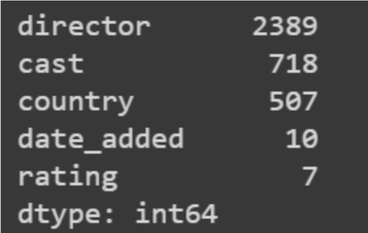
The variables having null values are director, cast, country, date_added, and rating.
description: summary of the description.
We cannot impute anything in place of these values. So, whenever we use any of the string object type variables we replace null values with empty spaces. And, when we use date_added we remove the observations containing null values.
We check if there is any kind of repetition of TV Shows in different seasons. This is done by getting the value counts of ‘type’ column to get the number of Movies and TV Shows in our dataset. Then we find the number of unique titles in TV-Shows. Since the number of TV-Shows in ‘type’ column and number of unique ‘titles’ in TV Shows are equal we verified that there is no repetition of TV Shows as different seasons.
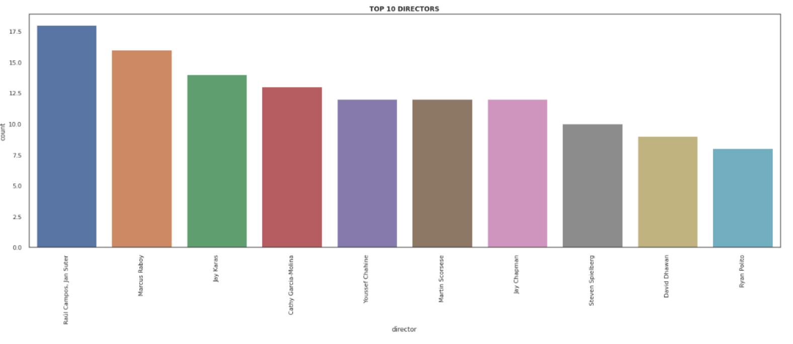
The top 10 directors by the number of contents directed are obtained by performing value counts on the director column and further using seaborn countplot to get the plot of the top 10 directors.
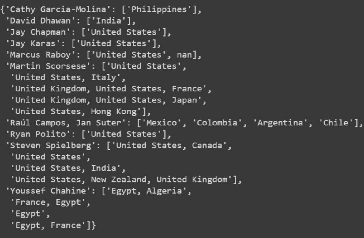
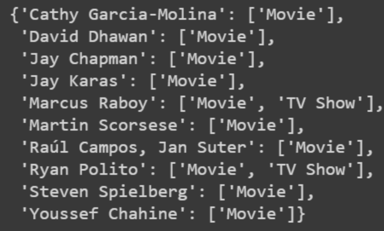
We store the top directors in a list, then for each entry in this list, we make two dictionaries where keys are the director's names and values are the genres of content directed by the directors and the country.
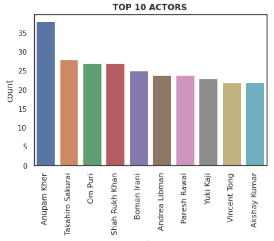
The actors are in the columns cast; for each observation, there is more than one entry separated by a comma. So, we make a list of all the values in the cast then we perform a countplot on it considering the top 10 actors.
Next, we perform a countplot on the country column to get the top 10 countries in which movies available on netflix are produced.
From the datetime column, date_added we extract the month and append it to a new column called month_added for each observation. Next, we perform a countplot on the month added column to get our plot containing months on x-axis and the number of movies released that month on y-axis.
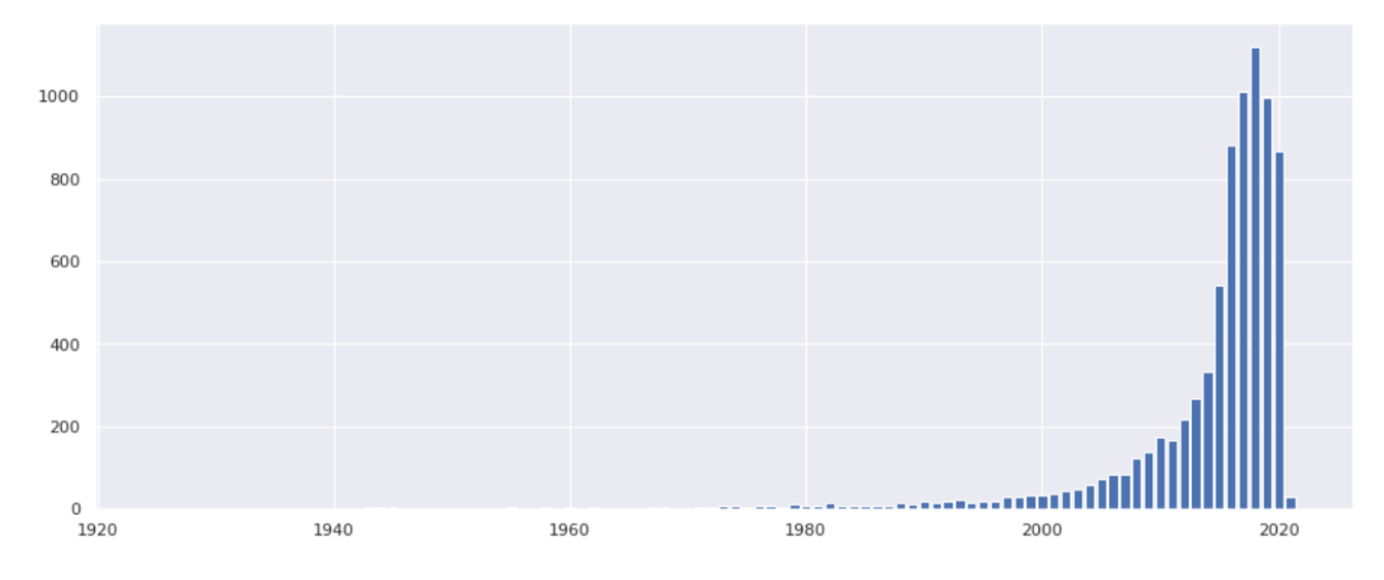
First, we visualise how many movies from each year is present in our dataset. For this we plot the graph of years on x-axis and number of movies released on y-axis. Next to visualise how ratings of content has changed over the years, we divide the dataframe into two sub-datasets one containing only Movies and another containing only TV-Shows.
Then for each of these datasets we groupby on release year and rating and aggregate the count of rating. Then each entry is divided by the number of movies/TV-Shows released that year and then multiplied by 100 to get the percentage this is done by performing groupby operation again on release_year and using transform to perform the percentage operation. Then plot the dataframe.
Content can be categorised by type i.e., Movie or TV-Show, rating and genre. We are going to look into all of them.
We perform a groupby operation on country and rating, where for each rating we count how many times it appears in a country. Then for each rating we plot how many times it appears non zero times in a country.
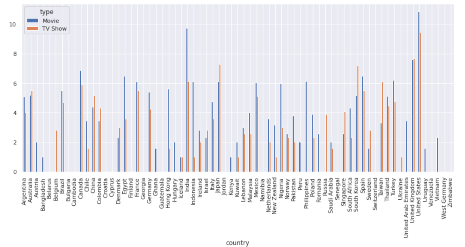
We perform a groupby operation on country and type and count the type for each country. Then we plot the dataframe but due to the large differences between the count values we perform a log2 operation.
The genres of any movie or tv show are stored in the listed_in column, where each genre is separated by a comma. So, first we make a column genre which contains the list of all genres a content belongs to. The list is obtained by performing .split(‘,’) on the strings in the listed_in column.
Once the genres column is obtained we perform MultiLabelBinarizer on it, make the corresponding dataframe and merge it with the original one. Next, we make a dictionary where keys are the genres or labels of mutilabelbinrizer and values are the sum of the columns. This way for each genre we get the number of times it appears in the dataframe. This data is then plotted to get the desired result.
The given dataframe contains 7000 observations varying across 13 years, so in order to make any conclusions we conduct hypothesis testing.
H0(Null-Hypothesis)= Netflix is focusing on movies and TV-Shows equally.
p0=0.5
HA(Alternate-Hypothesis)= Netflix is focusing less on TV-Shows
pA<0.5
Here, p represents the proportion of movies released in a given year.
Observed proportion = 0.75
Test Statistic:
p-p0 / (sqrt(p(1-p)/n) ~ N(0,1)
In our case n=12, because we consider uploads from year 2008 to 2020.
Thus, we get z=1.73 and p(z<1.73) = 0.95.
Therefore we cannot reject the null hypothesis. Hence, Netflix may not be focusing less on movies.
We perform a groupby operation on country and type and count the type for each country. Then we plot the dataframe but due to the large differences between the count values we perform a log2 operation.
First we use only the listed_in and type column to recommend content of the same type and same genre. From listed_in we extract all the genres of a particular content and one-hot encode the type column. Now we define a function on the principles of k-Nearest neighbours. We store all the columns/variables of an observation in an n-dimensional plane, when a particular id number and number of contents to recommend is entered in the function, the function produces the contents of nearest cosine distances except the entered one. Next, we decide to use an enhanced dataset to recommend movies and cluster movies.
-
Rename the title column with ‘NAME’.
-
Fill null values in text columns with empty spaces.
-
Make a new column called text which contains director, cast, listed_in and description. (with space between them)
-
Next one hot encode the type, rating and country column such that any of them having less than 5 counts is not considered.
-
Remove punctuations, stopwords from the created ‘text’ column and changing all alphaets to lowercase.
-
Lemmatize words from the text column.
-
Apply countvectorizer on the text column with max = 0.9, min = 3, n_grams=(1,2), max_features = 5000, binary = True.
We implement DBScan on this improved dataset to perform clustering operation but the curse of high dimensionality caused it to not work properly.
We first create a 2-dimensional array of the text pre processed dataframe from type_movie to the end of columns. Next we write functions to find silhouette score and within cluster sum of squares and plot it for each value of k. Basically k-elbow visualizer. Now we plot the silhouette scores and plot the k-elbow plot for equally distanced values between 2 and 703, that distance is 100. Next, for the optimal value of k, we chose other values of k and plotted the silhouette score and plot the elbow plot for values near the optimal value of k, and settle for a k-value of 175. Next, we perform k-Means clustering on the pre-processed dataset. In the end, using the same functions as defined previously we form clusters and recommend movies with better results.
We have finally reached the end of our project after completing EDA and clustering. The recommender system made works really well and gives results similar to the actual Netflix app.