Recommendation systems traditionally have faced a problem of giving quality recommendations from sparse data. The pressure to answer this problem is vital for many companies that require proper recommendations to users as a way to drive engagement and sell products. In this project we have used the Movielens 100K Dataset and try to give users the best recommendations possible.
Before we use a new neural network to solve our problem, let's assess the value of existing baseline techniques. The naive baye's classifier is one of the oldest, most reliable methods to this day.
Naive Bayes is a supervised machine learning algorithm that is used in classification problems. The algorithm is based on the Bayes theorem of probability.
P(A|B) = P(B|A)P(A)P(B)
Using Bayes theorem, we can find the probability of A happening, given that B has occurred. Here, B is the evidence and A is the hypothesis. The assumption made here is that the predictors/features are independent. We assume one particular feature does not affect the other, hence the name "Naive".
We have used this to make a recommendation system as the naive bayes classifier does a fantastic job in classification problems related to text based datasets. Naive Bayes classifiers and collaborative filtering together builds a recommendation system that uses machine learning and data mining techniques to filter unseen information and predict whether a user would like a given resource or not.
When Netflix was starting to take off, it came into a problem of trying to find optimal movies to recommend to customers. This sparked a million dollar challenge to find the best algorithm for the purpose of recommending movies. The winner was Matrix Factorization; a new method to embed users and recommend the best movie possible.
In data science, low-rank matrix factorization (MF) is a crucial method. The fundamental tenet of MF is that there are latent structures in the data that may be revealed in order to produce a compressed representation of the data. The MF method offers a unified approach for dimension reduction, clustering, and matrix completion by factorizing an initial matrix to low-rank matrices.
MF has a number of appealing characteristics, including the following:
- It reveals latent structures in the data while addressing the data sparseness problem.
- It has an elegant probabilistic interpretation.
- It is easily extended with domain-specific prior knowledge (for example, homophily in linked data), making it appropriate for a variety of real-world problems.
- It is possible to use many optimization techniques, such as stochastic gradient-based methods, to find a suitable solution.
When we factorize a matrix, we essentially divide it into two smaller matrices, each with a smaller dimension. These matrices are commonly referred to as "Embeddings." Variants of matrix factorization include "Low Rank MF" and "Non-Negative MF".
In the code, we've employed a technique known as "Low Rank Matrix Factorization." We have produced embeddings for both the user and the item, in this example the movie. In this application of collaborative filtering, the number of dimensions or the so-called "Latent Factors" in the embeddings is a hyperparameter to deal with.
The new method making use of machine learning is called a JNCF Recommender based off of this paper. This paper takes a user's rating of every item, a liked item's rating by every user, and an unknown (negative) item's rating by every user. A positive sample in training is a sample that has a rating, a negative sample is a sample that wasn't rated by the user. We feed both of these types of items into our model because it's important to understand not only what a user has seen and therefore shown interest in, but also what a user hasn't seen and is less likely to enjoy.
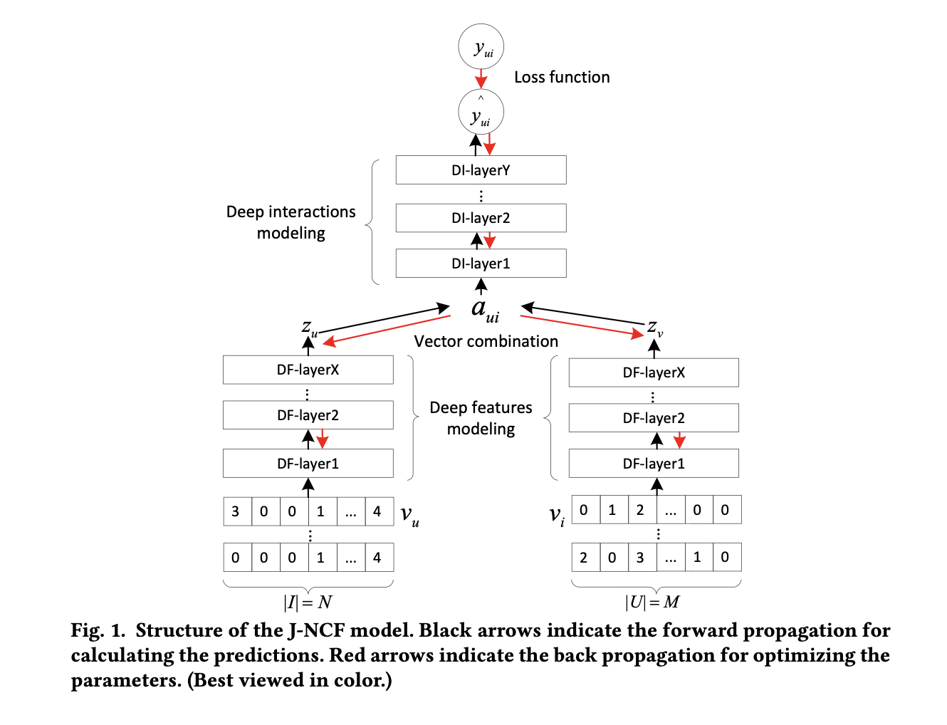
The image above shows these vectors being fed into a deep feature embedding network whose job is to create latent representations of each vector through multiple ReLU layers. Then the two embeddings are concatenated and fed into a deep interaction network that looks at the connections between user and item and decides the likelihood that a user will enjoy this movie.

The following describes the loss function for our algorithm. The constant balances the importance of pair-wise and point-wise loss functions. Pair-wise loss takes into account how well the positive item was ranked above the negative item, and point-wise loss assesses how well the positive item was rated according to its ground truth (gt). This is a hybrid loss function that works exceptionally well at tuning the model. We tried many other methods by which one could try to assess loss but the author's hybrid loss function was always superior. Focusing either on entirely pairwise loss or point wise estimation, or any other blend gave worse results.
For evaluating the efficiency of the model, the recommendation system community opts to use 99 negative samples and one positive sample, as the relative accuracy doesn't change, but the overall accuracy does along with a decreased evaluation time. This leads to much faster results at the cost of misleading some readers into thinking an algorithm performs better than it truly does using the entire dataset. Our model gave a 53% hit rate of the top 10 (HR@10) when using only 100 examples, while when using the entire item list we only got 21% HR@10. In practice this may not be that big of a deal, as recommender systems often only use neural networks for top results, and let simpler algorithms determine which results are even evaluated by the model. So in reality, this isn't as big of a deal as one might think. For reference, our Low Rank Matrix Factorization HR@10 was only 37%, meaning from our baseline, our increase in hit rate grew by 16%! If only we could go back to 2009 and win that million dollar Netflix prize!
Even though we saw a drastic improvement in accuracy, the accuracy the paper describes is much greater. The reason this is the case is hard to say, but many possibilities come up. The most important one being that of unclear hyperparameter tuning the authors underwent without fully explaining. For the same model, the original authors of the paper got 68% HR@10, 15% better than my model. The hyperparameters involved are learning rate, negative sample size, batch size, epochs, layer sizes and the loss function's alpha constant. I also used a normalized dataset rather than the paper that doesn't normalize ratings between 0 and 1. They instead use a sigmoid at the end of the model, however when implementing this change I saw a decrease in accuracy for my model, so I opted for my method of normalizing my dataset before training as it was faster and gave better accuracy.