Exercise on Identification of patterns of statistical control charts with use of artificial neural networks.
In the present exercise we were asked to approach the SPC (Statistical Process Control) pattern approach and the automatic recognition by TND. Our initial approach was to understand the simple and the complex patterns, as well as our familiarity with Western Electric rules (These rules detect out-of-control or non-random patterns in control charts). The languages programming we chose to use is Python for production and data presentation, R programming language for use and familiarity with standards Western Electric and finally the MatLab program for the creation and training of the Artificial Neural Network.
The logic we followed was to create 20 point patterns between the ± 3 values. Specifically the simple patterns Uptrend, Stratification, Point Outside of Control Limits and Instability were created. In addition, the complex Cycle and Instability and Instability and Grouping patterns were created. The way their creation was as follows:
- Create a 20-dot pattern for each type of pattern we will use (Uptrend, Stratification, ...., Instability and Grouping) with values that we type manually.
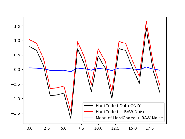
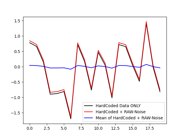
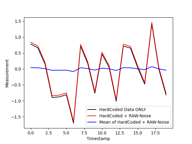
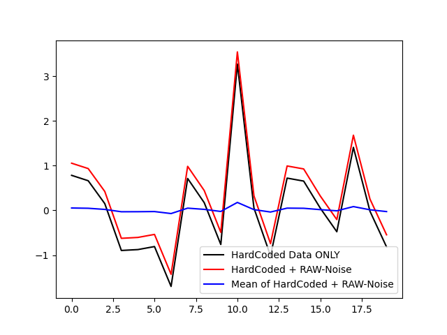
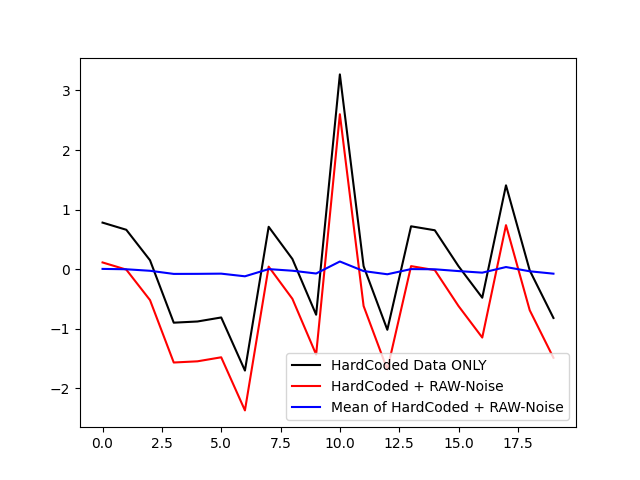
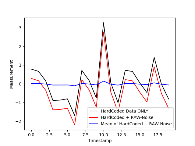
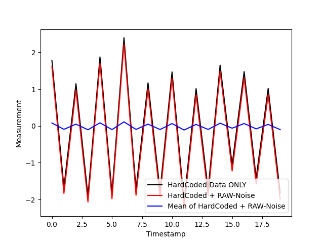
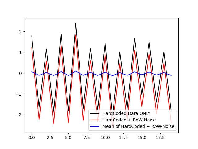
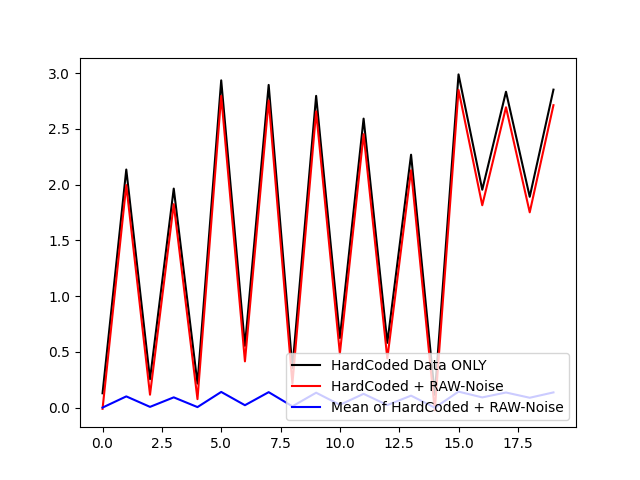
- Automatic production of 1000 patterns for each of them added to them so White Noise as well as random noise from Gaussian distribution (Figures 1 to 6 graphic representation of the manual pattern in relation to what is produced that has been added randomness). The final Dataset created is 6000 sample patterns.
- In each of them, an average of 20 points is calculated for four parameters of each pattern (Mean), minimum and maximum value (min, max) and curvature (Kurtosis) as defined by Fisher. It is worth noting that others can be added calculations in future implementation if the Python Pandas library offers us a variety of options. Therefore the current state of our dataset is an array dimensions 6000x24.
- For the 6 patterns we have, a dataset with the targets should be created which will be binary. This will be in the format 6000x6. Structure:
Stratification Pattern = 1 0 0 0 0 0
Uptrend = 0 1 0 0 0 0
Instability = 0 0 1 0 0 0
Point Outside of Control Limits = 0 0 0 1 0 0
Cycle and Instability = 0 0 0 0 0 1 1 0
Instability and Grouping = 0 0 0 0 0 1
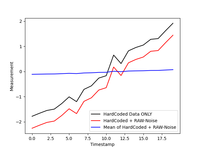
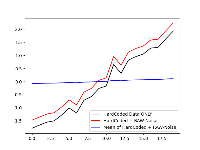
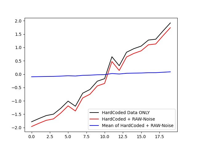
(Figure 1 Examples of data generation for pattern: Uptrend)
 )
)
(Figure 2 Examples of pattern data creation: Stratification)
(Figure 3 Examples of pattern data generation: Point Outside Of Control)

(Figure 4 Examples of data creation for pattern: Instability)
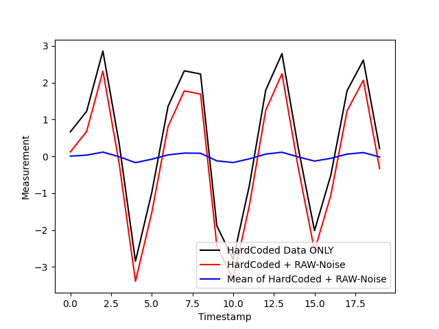
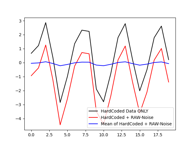
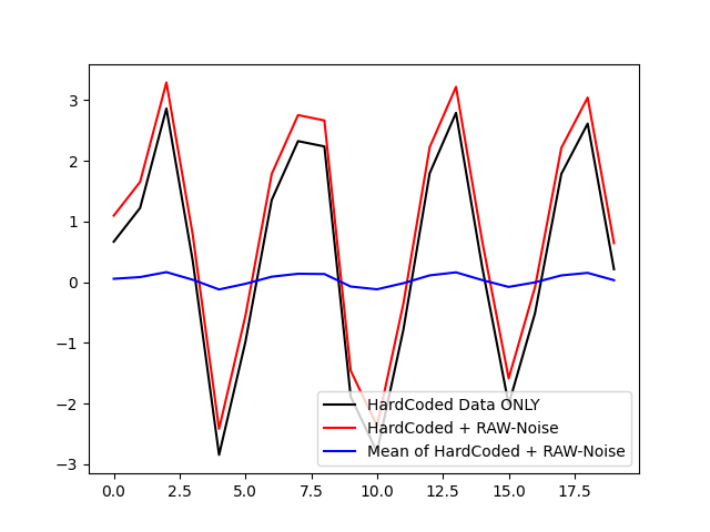
(Figure 5 Examples of data generation for pattern: Cycle and Instability)
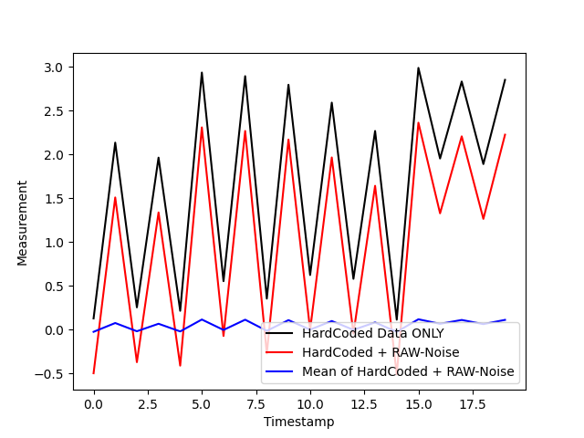
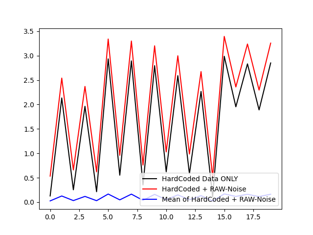
(Figure 6 Examples of data creation for pattern: Instability and Grouping)
The TND was created using MatLab's Neural Pattern Recognition library. We have selected this tool for the ease of use it offers as well as the plethora of options. Below we see the steps we followed to create 2 TND. The only difference two TNDs is that one consists of one Hidden Layer and the other of two (Figure 7). Education of TND was done with a percentage of 80-5-15, ie 4800 training data, 300 validation data and 900 testing data (Figure 8).
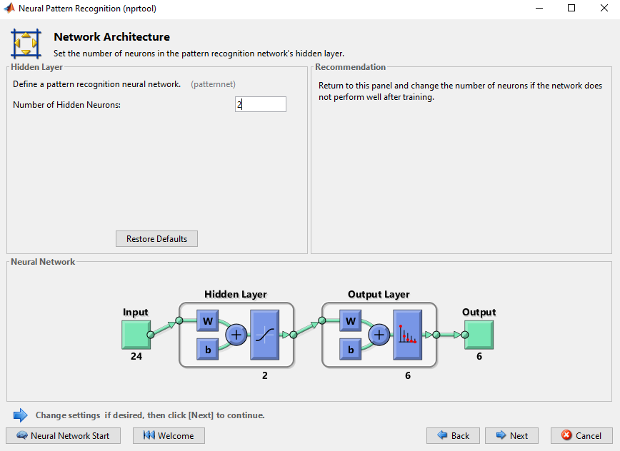
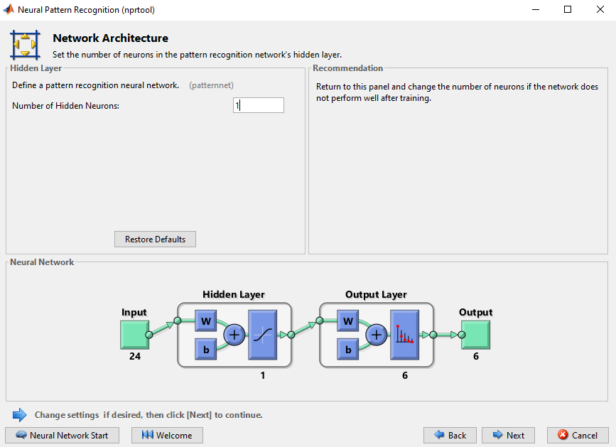
(Figure 7 Architecture of the two ANNs)
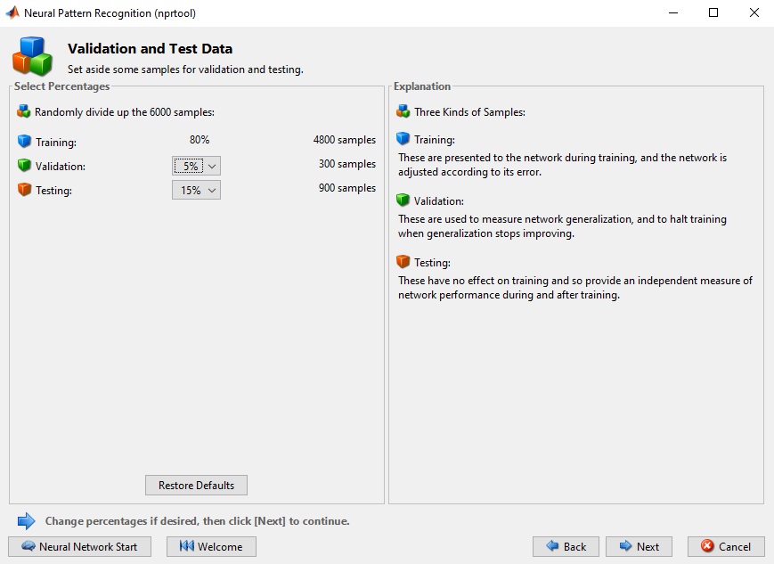
(Figure 8 training data structure)
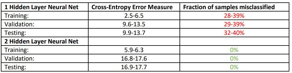
After training both ANNs we came to the following range of results (Figures 9-13 contain a simulation for each ANN):
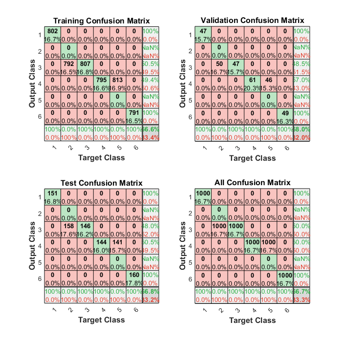
(Figure 9 Plot Confusion for NN with one Hidden Layer)
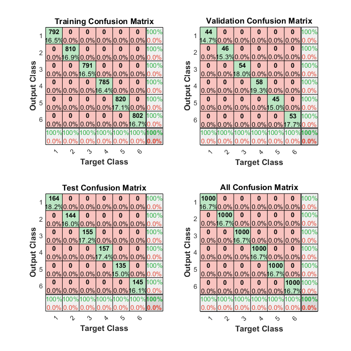
(Figure 10 Plot Confusion for NN with two Hidden Layers)
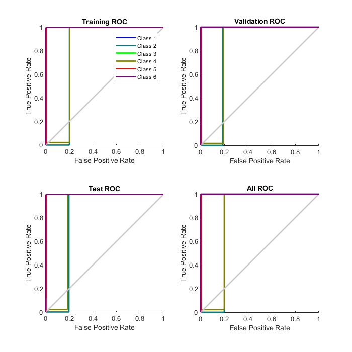
(Figure 11 Plot ROC for NN with a Hidden Layer)
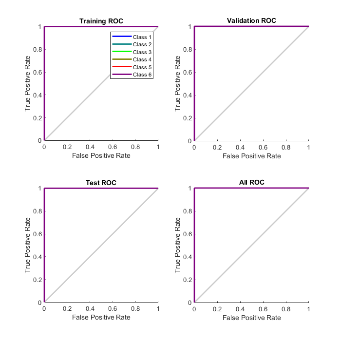
(Figure 12 Plot ROC for NN with two Hidden Layers)
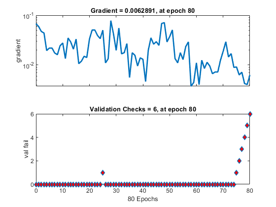
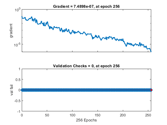
(Figure 13 Training state of Neural Nets Gradients in correlation with epochs for 1 Layer and 2 Layers)
The two ANNs gave us quite reliable results and we did not detect any signs of overfitting, however providing more patterns both simple and complex would definitely make ANN more demanding. Additionally we notice that the ANN with a Hidden Layer, has mainly the difficulty in separating Class 3-4-6 (Instability, Point Outside of Control Limits and Instability and Grouping) patterns which have the most similarities between them. One of future upgrades that could make our system more reliable would be extraction of primary patterns from real processing machines. Finally it is quite easy with the structure of our program in Python to add a variety of other methods data for patterns such as UCL, LCL and feature addition (median, percentage change between the current and a prior element etc.)