Image-processing

1. Develop a program to display grayscae image using read and write operations

import cv2
img=cv2.imread('f2.jpg',0)
cv2.imshow('image',img)
cv2.waitKey(0)
cv2.destroyAllwindows()

OUTPUT:

---

2. Develop a program to display the image using matplotlib

import matplotlib.image as mpimg
import matplotlib.pyplot as plt
img=mpimg.imread('b1.jpg')
plt.imshow(img)

OUTPUT:

---

3.Develop a program to perform linear transformation -Rotation

from PIL import Image
img=Image.open("b1.jpg")
img=img.rotate(180)
img.show()
cv2.waitKey(0)
cv2.destroyAllWindows()

OUTPUT:

---

4.Develop a program to convert color strings to RGB color values

from PIL import ImageColor
img1=ImageColor.getrgb("yellow")
print(img1)
img2=ImageColor.getrgb("red")
print(img2)

OUTPUT:
(255, 255, 0)
(255, 0, 0)

---

5.Write a program to create image using colors from PI import Image

from PIL import Image
img=Image.new('RGB',(200,400),(255,255,0))
img.show()

OUTPUT:

---

6.Develop a program to visualize the image using various colorspaces

import cv2
import matplotlib.pyplot as plt
import numpy as np
img=cv2.imread('b1.jpg')
plt.imshow(img)
plt.show()
img=cv2.cvtColor(img,cv2.COLOR_BGR2RGB)
plt.imshow(img)
plt.show()
img=cv2.cvtColor(img,cv2.COLOR_RGB2HSV)
plt.imshow(img)
plt.show()

OUTPUT:

---

7.Write a program to display the image attributes from PIL import Image

image=Image.open('b1.jpg')
print("Fiename:",image.filename)
print("Format:",image.format)
print("Size:",image.size)
print("Mode:",image.mode)
print("Width:",image.width)
print("Height:",image.height)
image.close();

OUTPUT:
Fiename: b1.jpg
Format: JPEG
Size: (1300, 1036)
Mode: RGB
Width: 1300
Height: 1036

---

8.Convert the original image to Gray scale and then to Binary

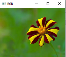
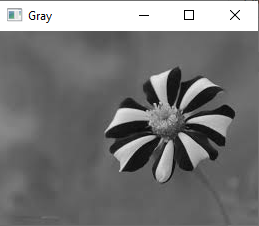
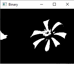
import cv2
img=cv2.imread('f1.jpg')
cv2.imshow("RGB",img)
cv2.waitKey(0)

img=cv2.imread('f1.jpg',0)
cv2.imshow("Gray",img)
cv2.waitKey(0)

ret,bw_img=cv2.threshold(img,127,255,cv2.THRESH_BINARY)
cv2.imshow("Binary",bw_img)
cv2.waitKey(0)
cv2.destroyAllWindows()

OUTPUT:

---

9.Resize the original image

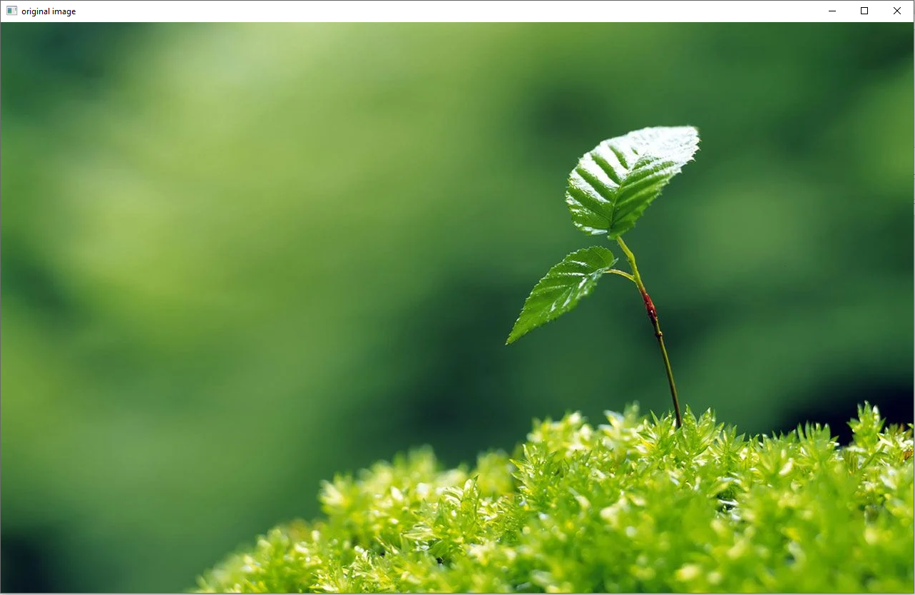
import cv2
img=cv2.imread('p1.jpg')
print('original image lenght width',img.shape)
cv2.imshow('original image',img)
cv2.waitKey(0)
imgresize=cv2.resize(img,(150,160))
cv2.imshow('Resized image',imgresize)
print('Resized image length width',imgresize.shape)
cv2.waitKey(0)

OUTPUT:
original image lenght width (800, 1280, 3)

---

1.Develop a program to read image using URL

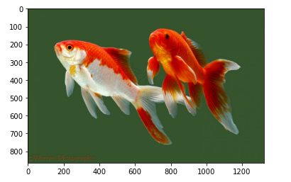
from skimage import io
import matplotlib.pyplot as plt
url='https://www.teahub.io/photos/full/41-417562_goldfish-fish-facts-wallpapers-pictures-download-gold-fish.jpg'
image=io.imread(url)
plt.imshow(image)
plt.show()

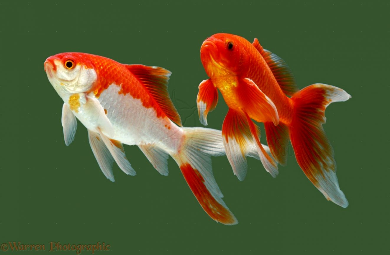
OUTPUT:

2.Write a program to mask and blur the image

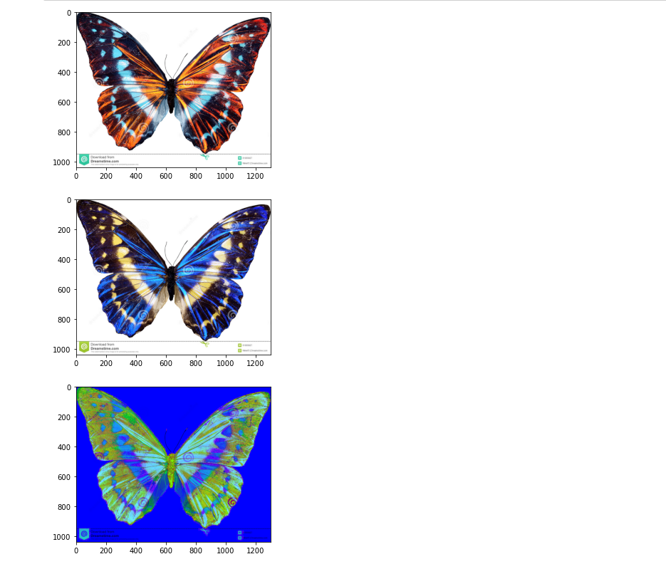
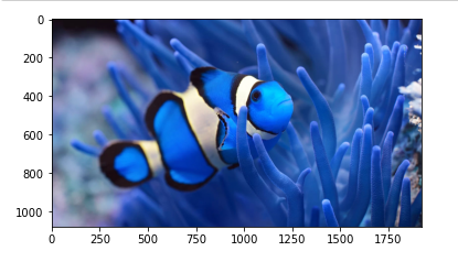
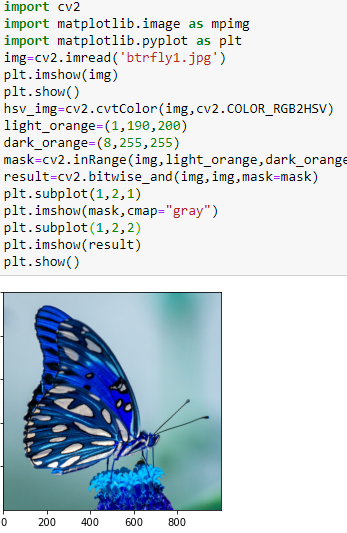
import cv2
import matplotlib.image as mpimg
import matplotlib.pyplot as plt
img=cv2.imread('fish.jpg')
plt.imshow(img)
plt.show()

OUTPUT:

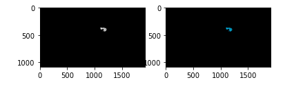
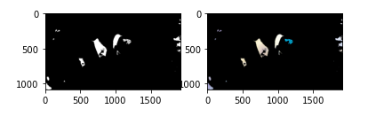
hsv_img=cv2.cvtColor(img,cv2.COLOR_RGB2HSV)
light_orange=(1,190,200)
dark_orange=(8,255,255)
mask=cv2.inRange(img,light_orange,dark_orange)
result=cv2.bitwise_and(img,img,mask=mask)
plt.subplot(1,2,1)
plt.imshow(mask,cmap="gray")
plt.subplot(1,2,2)
plt.imshow(result)
plt.show()

OUTPUT:

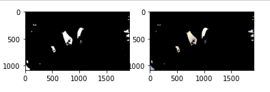
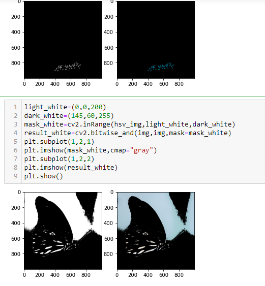
light_white=(0,0,200)
dark_white=(145,60,255)
mask_white=cv2.inRange(hsv_img,light_white,dark_white)
result_white=cv2.bitwise_and(img,img,mask=mask_white)
plt.subplot(1,2,1)
plt.imshow(mask_white,cmap="gray")
plt.subplot(1,2,2)
plt.imshow(result_white)
plt.show()

OUTPUT:

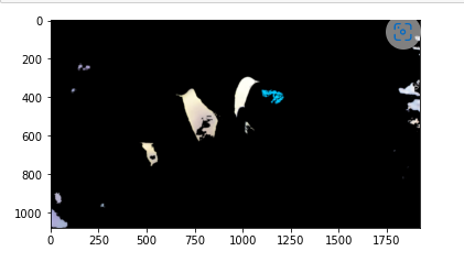
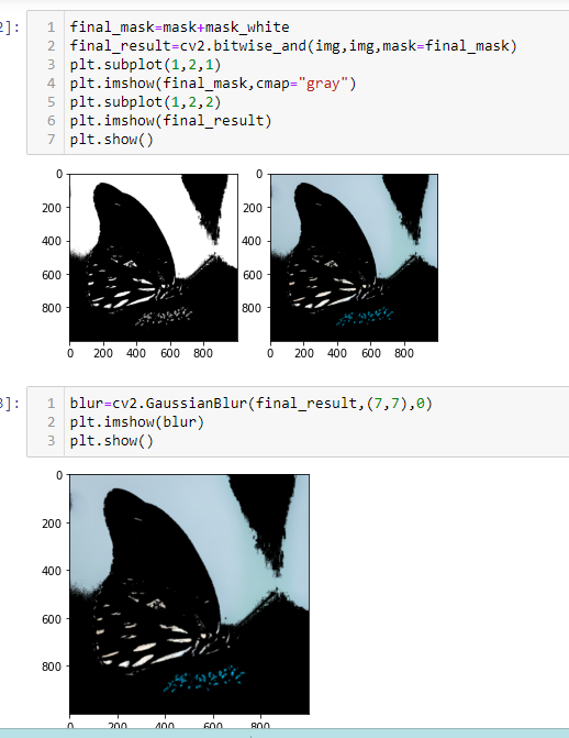
final_mask=mask+mask_white
final_result=cv2.bitwise_and(img,img,mask=final_mask)
plt.subplot(1,2,1)
plt.imshow(final_mask,cmap="gray")
plt.subplot(1,2,2)
plt.imshow(final_result)
plt.show()

OUTPUT:

blur=cv2.GaussianBlur(final_result,(7,7),0)
plt.imshow(blur)
plt.show()

OUTPUT:

---

NEW IMAGE

3.Write a program to perform arithmatic operations on images

import cv2
import matplotlib.image as mpimg
import matplotlib.pyplot as plt

img1=cv2.imread('f1.jpg')
img2=cv2.imread('f2.jpg')

fimg1 = img1 + img2
plt.imshow(fimg1)
plt.show()

cv2.imwrite('output.jpg',fimg1)
fimg2 = img1 - img2
plt.imshow(fimg2)
plt.show()

cv2.imwrite('output.jpg',fimg2)
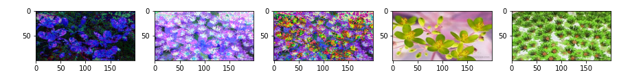
fimg3 = img1 * img2
plt.imshow(fimg3)
plt.show()

cv2.imwrite('output.jpg',fimg3)
fimg4 = img1 / img2
plt.imshow(fimg4)
plt.show()

cv2.imwrite('output.jpg',fimg4)

OUTPUT

4.Develop the program to change the image to different color space

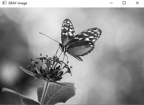
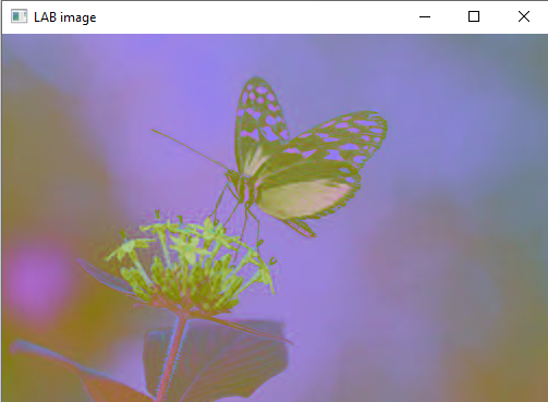
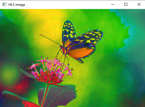
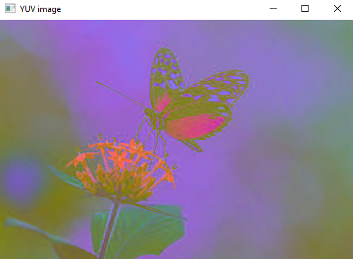
import cv2
img=cv2.imread('E:\b3.jpg')
gray=cv2.cvtColor(img,cv2.COLOR_BGR2GRAY)
hsv=cv2.cvtColor(img,cv2.COLOR_BGR2HSV)
lab=cv2.cvtColor(img,cv2.COLOR_BGR2LAB)
hls=cv2.cvtColor(img,cv2.COLOR_BGR2HLS)
yuv=cv2.cvtColor(img,cv2.COLOR_BGR2YUV)
cv2.imshow("GRAY image",gray)
cv2.imshow("HSV image",hsv)
cv2.imshow("LAB image",lab)
cv2.imshow("HLS image",hls)
cv2.imshow("YUV image",yuv)
cv2.waitKey(0)
cv2.destroyAllWindows()

OOUTPUT

5.Program to create an image using 2D array

import cv2 as c
import numpy as np
from PIL import Image
array=np.zeros([100,200,3],dtype=np.uint8)
array[:,:100] = [250,130,0]
array[:,100:] = [0,0,255]
img=Image.fromarray(array)
img.save('image1.png')
img.show()
c.waitKey(0)

OUTPUT

6.Bitwise Operation(with two diff images)

import cv2
import matplotlib.pyplot as plt
image1=cv2.imread('f3.jpg')
image2=cv2.imread('f4.jpg')
ax=plt.subplots(figsize=(15,10))
bitwiseAnd=cv2.bitwise_and(image1,image2)
bitwiseOr=cv2.bitwise_or(image1,image2)
bitwiseXor=cv2.bitwise_xor(image1,image2)
bitwiseNot_img1=cv2.bitwise_not(image1)
bitwiseNot_img2=cv2.bitwise_not(image2)
plt.subplot(151)
plt.imshow(bitwiseAnd)
plt.subplot(152)
plt.imshow(bitwiseOr)
plt.subplot(153)
plt.imshow(bitwiseXor)
plt.subplot(154)
plt.imshow(bitwiseNot_img1)
plt.subplot(155)
plt.imshow(bitwiseNot_img2)
cv2.waitKey(0)

OUTPUT

7.Bitwise Operation(with two same images)

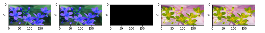
import cv2
import matplotlib.pyplot as plt
image1=cv2.imread('f3.jpg')
image2=cv2.imread('f3.jpg')
ax=plt.subplots(figsize=(15,10))
bitwiseAnd=cv2.bitwise_and(image1,image2)
bitwiseOr=cv2.bitwise_or(image1,image2)
bitwiseXor=cv2.bitwise_xor(image1,image2)
bitwiseNot_img1=cv2.bitwise_not(image1)
bitwiseNot_img2=cv2.bitwise_not(image2)
plt.subplot(151)
plt.imshow(bitwiseAnd)
plt.subplot(152)
plt.imshow(bitwiseOr)
plt.subplot(153)
plt.imshow(bitwiseXor)
plt.subplot(154)
plt.imshow(bitwiseNot_img1)
plt.subplot(155)
plt.imshow(bitwiseNot_img2)
cv2.waitKey(0)

OUTPUT

8.Blurring

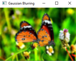
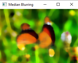
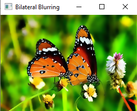
import cv2
import numpy as np
image=cv2.imread('B2.jpg')
cv2.imshow('Original Image',image)
cv2.waitKey(0)
Gaussian=cv2.GaussianBlur(image,(7,7),0)
cv2.imshow('Gaussian Blurring',Gaussian)
cv2.waitKey(0)
median=cv2.medianBlur(image,15)
cv2.imshow('Median Blurring',median)
cv2.waitKey(0)
bilateral=cv2.bilateralFilter(image,9,75,75)
cv2.imshow('Bilateral Blurring',bilateral)
cv2.waitKey(0)
cv2.destroyAllWindows()

OUTPUT

---

9.Image Enhancement

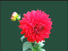
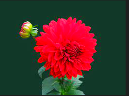
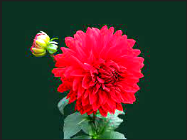
from PIL import Image
from PIL import ImageEnhance
image=Image.open('B2.jpg')
image.show()
enh_bri=ImageEnhance.Brightness(image)
brightness=1.5
image_brightened=enh_bri.enhance(brightness)
image_brightened.show()
enh_col=ImageEnhance.Color(image)
color=1.5
image_colored=enh_col.enhance(color)
image_colored.show()
enh_con=ImageEnhance.Contrast(image)
contrast=1.5
image_contrasted=enh_con.enhance(contrast)
image_contrasted.show()
enh_sha=ImageEnhance.Sharpness(image)
sharpness=3.0
image_sharped=enh_sha.enhance(sharpness)
image_sharped.show()

output

---

10.Morphology

import cv2
import numpy as np
from matplotlib import pyplot as plt
from PIL import Image,ImageEnhance
img=cv2.imread('B2.jpg',0)
ax=plt.subplots(figsize=(20,10))
kernel=np.ones((5,5),np.uint8)
opening=cv2.morphologyEx(img,cv2.MORPH_OPEN,kernel)
closing=cv2.morphologyEx(img,cv2.MORPH_CLOSE,kernel)
erosion=cv2.erode(img,kernel,iterations=1)
dilation=cv2.dilate(img,kernel,iterations=1)
gradient=cv2.morphologyEx(img,cv2.MORPH_GRADIENT,kernel)
plt.subplot(151)
plt.imshow(opening)
plt.subplot(152)
plt.imshow(closing)
plt.subplot(153)
plt.imshow(erosion)
plt.subplot(154)
plt.imshow(dilation)
plt.subplot(155)
plt.imshow(gradient)
cv2.waitKey(0)

OUTPUT

11.Original and Grayscale Image

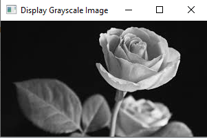
import cv2
OriginalImg=cv2.imread('img1.jpg')
GrayImg=cv2.imread('img1.jpg',0)
isSaved=cv2.imwrite('‪‪E:\flwr\img1.jpg',GrayImg)
cv2.imshow('Display Original Image',OriginalImg)
cv2.imshow('Display Grayscale Image',GrayImg)
cv2.waitKey(0)
cv2.destroyAllWindows()
if isSaved:
print('The image is successfully saved.')

OUTPUT*

12.Graylevel slicing with background

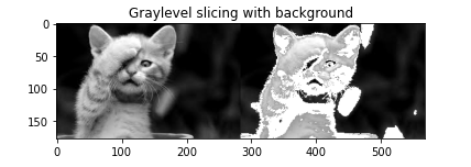
import cv2
import numpy as np
from matplotlib import pyplot as plt
image=cv2.imread('cat.jpg',0)
x,y=image.shape
z=np.zeros((x,y))
for i in range(0,x):
for j in range(0,y):
if(image[i][j]>50 and image[i][j]<150):
z[i][j]=255
else:
z[i][j]=image[i][j]
equ=np.hstack((image,z))
plt.title('Graylevel slicing with background')
plt.imshow(equ,'gray')
plt.show()

OUTPUT

13.Graylevel slicing without background

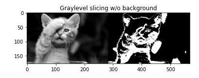
import cv2
import numpy as np
from matplotlib import pyplot as plt
image=cv2.imread('cat.jpg',0)
x,y=image.shape
z=np.zeros((x,y))
for i in range(0,x):
for j in range(0,y):
if(image[i][j]>50 and image[i][j]<150):
z[i][j]=255
else:
z[i][j]=0
equ=np.hstack((image,z))
plt.title('Graylevel slicing with background')
plt.imshow(equ,'gray')
plt.show()

OUTPUT

14.Analyse the image data using HISTOGRAM(numpy)

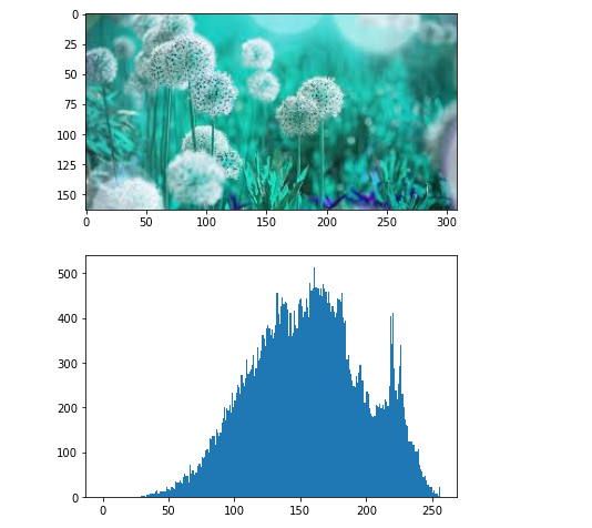
import numpy as np
import cv2 as cv
from matplotlib import pyplot as plt
img = cv.imread('n3.jpg')
plt.imshow(img)
plt.show()
img = cv.imread('n3.jpg',0)
plt.hist(img.ravel(),256,[0,256]);
plt.show()

OUTPUT

---

skimage

from skimage import io
import matplotlib.pyplot as plt
img = io.imread('n3.jpg')
plt.imshow(img)
plt.show()
image = io.imread('n3.jpg')
ax = plt.hist(image.ravel(), bins = 256)
plt.show()

OUTPUT

from skimage import io
import matplotlib.pyplot as plt
img = cv.imread('n3.jpg')
plt.imshow(img)
plt.show()
ax = plt.hist(image.ravel(), bins = 256)
ax = plt.xlabel('Intensity Value')
ax = plt.ylabel('Count')
plt.show()

OUTPUT

---

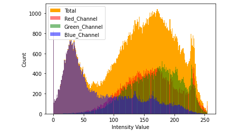
from skimage import io
import matplotlib.pyplot as plt
image = io.imread('n3.jpg')
_ = plt.hist(image.ravel(), bins = 256, color = 'orange', )
_ = plt.hist(image[:, :, 0].ravel(), bins = 256, color = 'red', alpha = 0.5)
_ = plt.hist(image[:, :, 1].ravel(), bins = 256, color = 'Green', alpha = 0.5)
_ = plt.hist(image[:, :, 2].ravel(), bins = 256, color = 'Blue', alpha = 0.5)
_ = plt.xlabel('Intensity Value')
_ = plt.ylabel('Count')
_ = plt.legend(['Total', 'Red_Channel', 'Green_Channel', 'Blue_Channel'])
plt.show()

OUTPUT

---

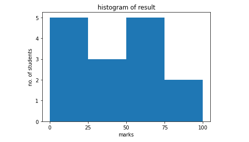
from matplotlib import pyplot as plt
import numpy as np
fig,ax = plt.subplots(1,1)
a = np.array([22,87,5,43,56,73,55,54,11,20,51,5,79,31,27])
ax.hist(a, bins = [0,25,50,75,100])
ax.set_title("histogram of result")
ax.set_xticks([0,25,50,75,100])
ax.set_xlabel('marks')
ax.set_ylabel('no. of students')
plt.show()

OUTPUT

15.Program to perform basic image data analysis using intensity transformation:

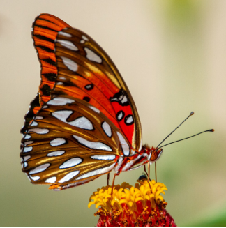
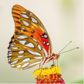
a) Image negative
b) Log transformation
c) Gamma correction

%matplotlib inline
import imageio
import matplotlib.pyplot as plt
import warnings
import matplotlib.cbook
warnings.filterwarnings("ignore",category=matplotlib.cbook.mplDeprecation)
pic=imageio.imread('btrfly1.jpg')
plt.figure(figsize=(6,6))
plt.imshow(pic);
plt.axis('off');

OUTPUT

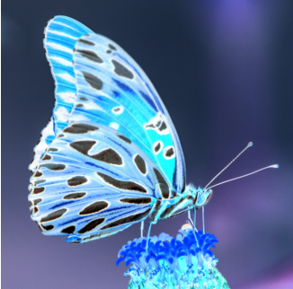
negative=255-pic
plt.figure(figsize=(6,6))
plt.imshow(negative);
plt.axis('off');

OUTPUT

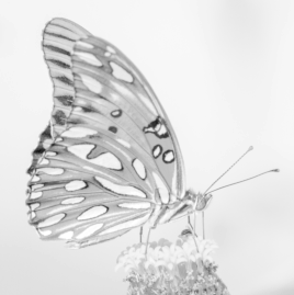
%matplotlib inline
import imageio
import numpy as np
import matplotlib.pyplot as plt
pic=imageio.imread('btrfly1.jpg')
gray=lambda rgb : np.dot(rgb[...,:3],[0.299,0.587,0.114])
gray=gray(pic)
max_=np.max(gray)
def log_transform():
return(255/np.log(1+max_))*np.log(1+gray)
plt.figure(figsize=(5,5))
plt.imshow(log_transform(),cmap=plt.get_cmap(name='gray'))
plt.axis('off');

OUTPUT

import imageio
import matplotlib.pyplot as plt
pic=imageio.imread('btrfly1.jpg')
gamma=2.2
gamma_correction=((pic/255)**(1/gamma))
plt.figure(figsize=(5,5))
plt.imshow(gamma_correction)
plt.axis('off');

OUTPUT

16.Program to perform basic image manipulation:

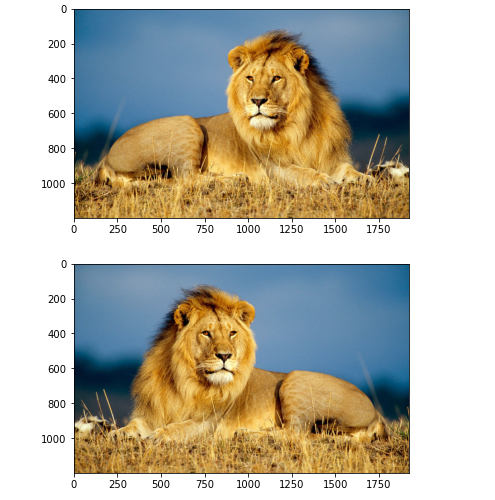
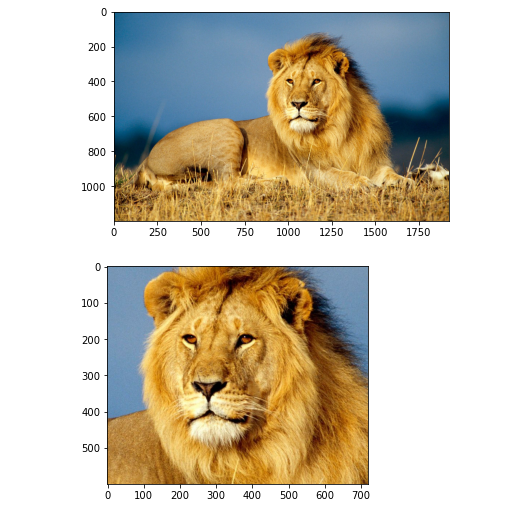
a) Sharpness
b) Flipping
c) Cropping

from PIL import Image
from PIL import ImageFilter
import matplotlib.pyplot as plt
my_image=Image.open('lion.jpg')
sharp=my_image.filter(ImageFilter.SHARPEN)
sharp.save('D:/lion_sharpen.jpg')
sharp.show()
plt.imshow(sharp)
plt.show()

OUTPUT

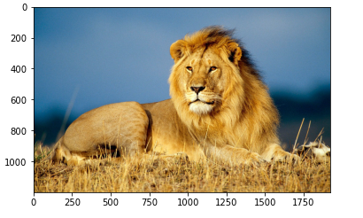
import matplotlib.pyplot as plt
img=Image.open('lion.jpg')
plt.imshow(img)
plt.show()
flip=img.transpose(Image.FLIP_LEFT_RIGHT)
flip.save('D:/lion_sharpen.jpg')
plt.imshow(flip)
plt.show()

OUTPUT

from PIL import Image
import matplotlib.pyplot as plt
im=Image.open('lion.jpg')
plt.imshow(im)
plt.show()
width,height=im.size
im1=im.crop((750,200,1600,800))
#im1.show()
plt.imshow(im1)
plt.show()

OUTPUT
\

from PIL import Image
import numpy as np
w, h =512,512
data = np.zeros((h, w, 3), dtype=np.uint8)
data[0:256, 0:256] = [255, 0, 0] # red patch in upper left
img = Image.fromarray(data, 'RGB')
img.save('my.png')
img.show()

OUTPUT

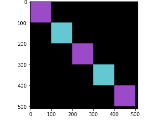
from PIL import Image
import matplotlib.pyplot as plt
import numpy as np
w, h = 512,512
data = np.zeros((h, w, 3), dtype=np.uint8)
data[0:100, 0:100] = [155, 75, 200]
data[100:200,100:200] = [100,200,210]
data[200:300,200:300 ] = [155, 75, 200]
data[300:400,300:400] = [100,200,210]
data[400:500, 400:500] = [155, 75, 200]
#red patch in upper left
img = Image.fromarray(data, 'RGB')
#img.save('my.png')
#img.show()
plt.imshow(img)
plt.show()

OUTPUT

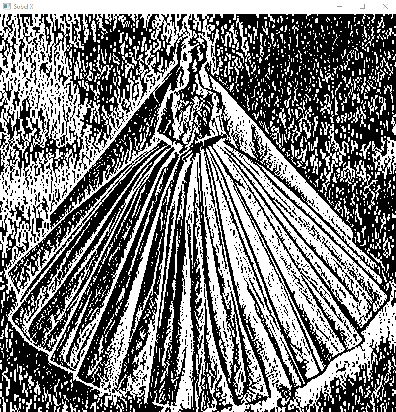
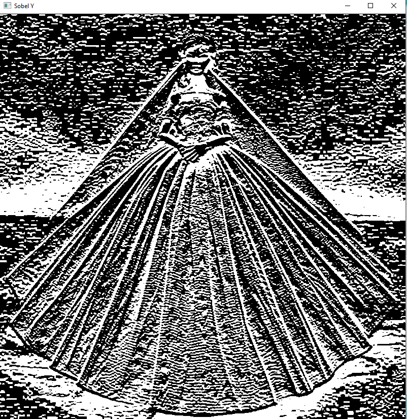
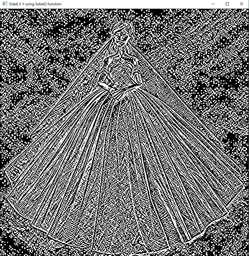
EDGE DETECTION:
import cv2
#Read the original image
img = cv2.imread('B1.jpg')
#Display original image
cv2.imshow('Original', img)
cv2.waitKey(0)
#Convert to graycsale
img_gray = cv2.cvtColor(img, cv2.COLOR_BGR2GRAY)
#Blur the image for better edge detection
img_blur = cv2.GaussianBlur(img_gray, (3,3), 0)
#Sobel Edge Detection
sobelx = cv2.Sobel(src=img_blur, ddepth=cv2.CV_64F, dx=1, dy=0, ksize=5) # Sobel Edge Detection on the X axis
sobely = cv2.Sobel(src=img_blur, ddepth=cv2.CV_64F, dx=0, dy=1, ksize=5) # Sobel Edge Detection on the Y axis
sobelxy = cv2.Sobel(src=img_blur, ddepth=cv2.CV_64F, dx=1, dy=1, ksize=5) # Combined X and Y Sobel Edge Detection
#Display Sobel Edge Detection Images
cv2.imshow('Sobel X', sobelx)
cv2.waitKey(0)
cv2.imshow('Sobel Y', sobely)
cv2.waitKey(0)
cv2.imshow('Sobel X Y using Sobel() function', sobelxy)
cv2.waitKey(0)
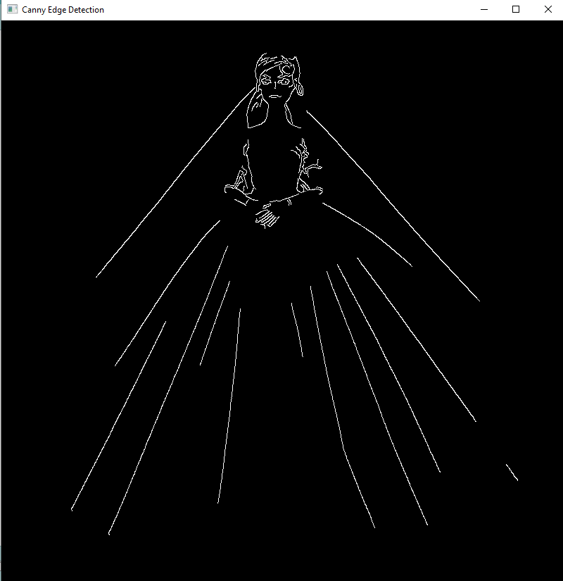
#Canny Edge Detection
edges = cv2.Canny(image=img_blur, threshold1=100, threshold2=200) # Canny Edge Detection
#Display Canny Edge Detection Image
cv2.imshow('Canny Edge Detection', edges)
cv2.waitKey(0)
cv2.destroyAllWindows()

OUTPUT:

USING PILLOW FUNCTIONS

from PIL import Image, ImageChops, ImageFilter
from matplotlib import pyplot as plt
#Create a PIL Image objects
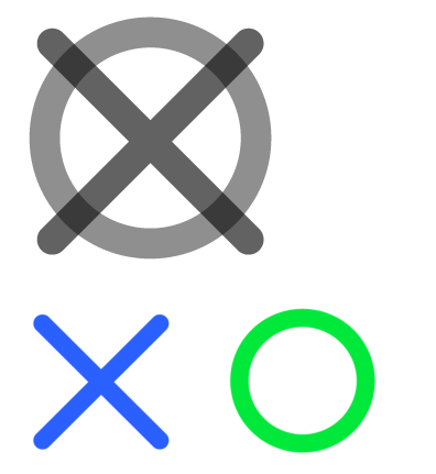
x = Image.open("x.png")
o = Image.open("o.png")
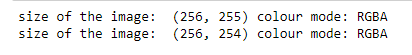
#Find out attributes of Image Objects
print('size of the image: ', x.size, ' colour mode:', x.mode)
print('size of the image: ', o.size, ' colour mode:', o.mode)
#plot 2 images one besides the other
plt.subplot(121), plt.imshow(x)
plt.axis('off')
plt.subplot(122), plt.imshow(o)
plt.axis('off')
#multiply images
merged = ImageChops.multiply(x,o)
#adding 2 images
add = ImageChops.add(x,o)
#convert colour mode
greyscale = merged.convert('L')
greyscale

OUTPUT

#More Attributes
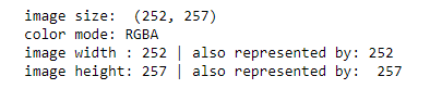
image = merged
print('image size: ', image.size, '\ncolor mode:', image.mode, '\nimage width :',image.width, '| also represented by:', image.size[0],
'\nimage height:',image.height, '| also represented by: ', image.size[1],)

#mapping the pixels of the image so we can use them as coordinates
pixel = greyscale.load()

#a nested Loop to parse through all the pixels in the image
for row in range(greyscale.size[0]):
for column in range(greyscale.size[1]):
if pixel[row, column] != (255):
pixel[row, column] = (0)
greyscale

#1. invert image
invert = ImageChops.invert(greyscale)
#2. invert by subtraction
bg = Image.new('L', (256, 256), color=(255)) #create a new image with a solid white background
subt = ImageChops.subtract(bg, greyscale) #subtract image from background
#3. rotate
rotate = subt.rotate(45)
rotate

#gaussian blur
blur = greyscale.filter(ImageFilter.GaussianBlur(radius=1))
#edge detection
edge = blur.filter(ImageFilter.FIND_EDGES)
edge

#change edge colours

edge = edge.convert('RGB')
bg_red = Image.new('RGB', (256,256), color = (255,0,0))
filled_edge = ImageChops.darker(bg_red, edge)
filled_edge

IMAGE RESTORATION

(a)Restore a damaged image

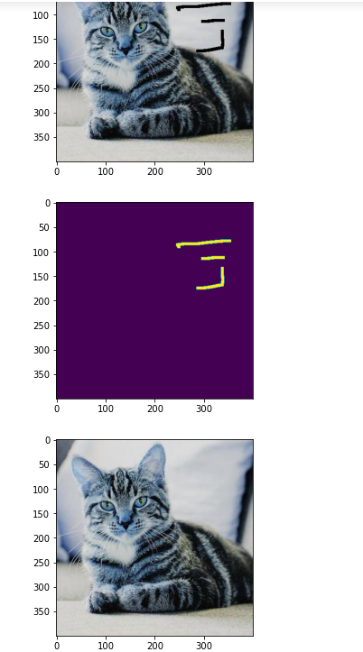
import numpy as np import cv2 import matplotlib.pyplot as plt #Open the image. img = cv2.imread('cat_damaged.png') plt.imshow(img) plt.show() #Load the mask. mask = cv2.imread('cat_mask.png', 0) plt.imshow(mask) plt.show() #Inpaint. dst = cv2.inpaint (img, mask, 3, cv2.INPAINT_TELEA) #write the output. cv2.imwrite('dimage_inpainted.png', dst) plt.imshow(dst) plt.show()

OUTPUT

(b)Removing Logos

import numpy as np
import matplotlib.pyplot as plt
import pandas as pd
plt.rcParams['figure.figsize'] = (10, 8)

def show_image (image, title='Image', cmap_type='gray'):
plt.imshow(image, cmap=cmap_type)
plt.title(title)
plt.axis('off')
def plot_comparison(img_original, img_filtered, img_title_filtered):
fig, (ax1, ax2)= plt.subplots (ncols=2, figsize=(10, 8), sharex=True, sharey=True)
ax1.imshow(img_original, cmap=plt.cm.gray)
ax1.set_title('Original')
ax1.axis('off')
ax2.imshow(img_filtered, cmap=plt.cm.gray)
ax2.set_title(img_title_filtered)
ax2.axis('off')

from skimage.restoration import inpaint
from skimage.transform import resize
from skimage import color

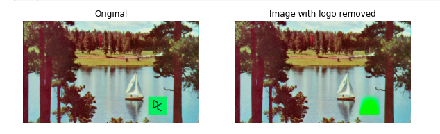
image_with_logo= plt.imread('imglogo.png')
#Initialize the mask
mask= np.zeros(image_with_logo.shape[:-1])
#Set the pixels where the Logo is to 1
mask [210:272, 360:425] = 1
#Apply inpainting to remove the Logo
image_logo_removed = inpaint.inpaint_biharmonic (image_with_logo,mask, multichannel=True)
#Show the original and Logo removed images
plot_comparison (image_with_logo, image_logo_removed, 'Image with logo removed')
OUTPUT

2)Noise

(a)Adding noise

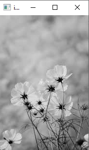
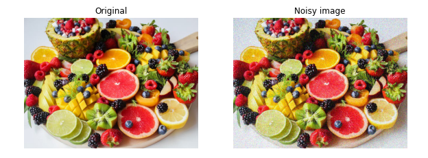
from skimage.util import random_noise
fruit_image = plt.imread('fruitts.jpeg')
#Add noise to the image
noisy_image = random_noise (fruit_image)
#Show th original and resulting image
plot_comparison (fruit_image, noisy_image, 'Noisy image')
OUTPUT

(b)Reducing Noise

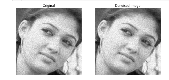
from skimage.restoration import denoise_tv_chambolle
noisy_image = plt.imread('noisy.jpg')
#Apply total variation filter denoising
denoised_image = denoise_tv_chambolle (noisy_image, multichannel=True)
#Show the noisy and denoised image
plot_comparison (noisy_image, denoised_image, 'Denoised Image')

(c)Reducing Noise while Preserving edges

from skimage.restoration import denoise_bilateral
landscape_image = plt.imread('noisy.jpg')
#Apply bilateral filter denoising
denoised_image = denoise_bilateral (landscape_image, multichannel=True)
#Show original and resulting images
plot_comparison (landscape_image, denoised_image, 'Denoised Image')
OUTPUT

3)Segmentation

(a)Superpixel segmentation

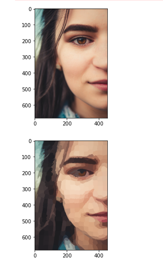
from skimage.segmentation import slic
from skimage.color import label2rgb
import matplotlib.pyplot as plt
import numpy as np
face_image = plt.imread('face.jpg')
segments = slic(face_image, n_segments=400)
segmented_image=label2rgb(segments,face_image,kind='avg')
plt.imshow(face_image)
plt.show()
plt.imshow((segmented_image * 1).astype(np.uint8))
plt.show()
OUTPUT

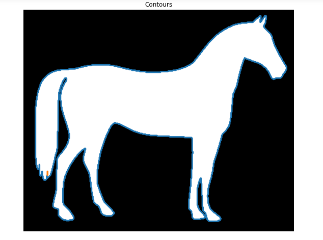
def show_image_contour (image, contours):
plt.figure()
for n, contour in enumerate(contours):
plt.plot(contour[:, 1], contour[:, 0], linewidth=3)
plt.imshow(image, interpolation='nearest', cmap='gray_r')
plt.title('Contours')
plt.axis('off')

from skimage import measure, data
#Obtain the horse image
horse_image = data.horse()
#Find the contours with a constant Level value of 0.8
contours = measure.find_contours (horse_image, level=0.8)
#Shows the image with contours found
show_image_contour (horse_image, contours)
OUTPUT

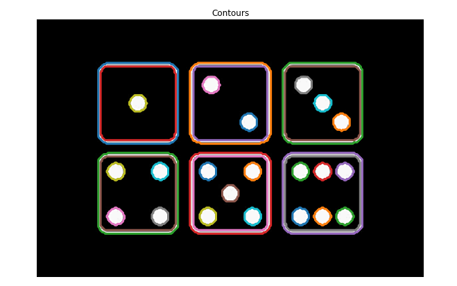
from skimage.io import imread
from skimage.filters import threshold_otsu
image_dices = imread('diceimg.png')
#Make the image grayscale
image_dices = color.rgb2gray(image_dices)
#obtain the optimal thresh value
thresh = threshold_otsu(image_dices)
#Apply thresholding
binary = image_dices > thresh
#Find contours at a constant value of 0.8
contours = measure.find_contours (binary, level=0.8)
#Show the image
show_image_contour (image_dices, contours)
OUTPUT

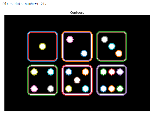
#Create List with the shape of each contour
shape_contours = [cnt.shape[0] for cnt in contours]
#Set 50 as the maximum size of the dots shape
max_dots_shape = 50
#Count dots in contours excluding bigger than dots size
dots_contours = [cnt for cnt in contours if np.shape(cnt)[0] < max_dots_shape]
#Shows all contours found
show_image_contour (binary, contours)
#Print the dice's number
print('Dices dots number: {}.'.format(len (dots_contours)))
OUTPUT

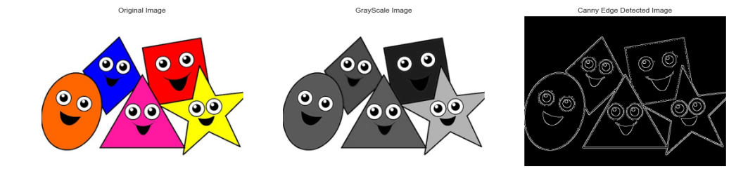
Implement a program to perform various edge detection techniques
a) Canny Edge detection
#Canny Edge detection
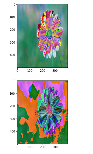
import cv2
import numpy as np
import matplotlib.pyplot as plt
plt.style.use('seaborn')
loaded_image = cv2.imread("Image.png")
loaded_image = cv2.cvtColor(loaded_image,cv2.COLOR_BGR2RGB)
gray_image = cv2.cvtColor(loaded_image, cv2.COLOR_BGR2GRAY)
edged_image = cv2.Canny(gray_image, threshold1=30, threshold2=100)
plt.figure(figsize=(20,20))
plt.subplot(1,3,1)
plt.imshow(loaded_image, cmap="gray")
plt.title("Original Image")
plt.axis("off")
plt.subplot(1,3,2)
plt.imshow(gray_image, cmap="gray")
plt.axis("off")
plt.title("GrayScale Image")
plt.subplot(1,3,3)
plt.imshow(edged_image,cmap="gray")
plt.axis("off")
plt.title("Canny Edge Detected Image")
plt.show()
OUTPUT

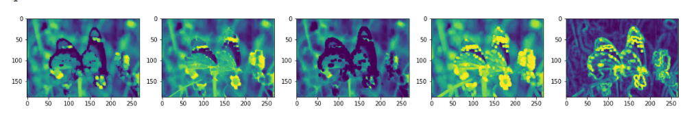
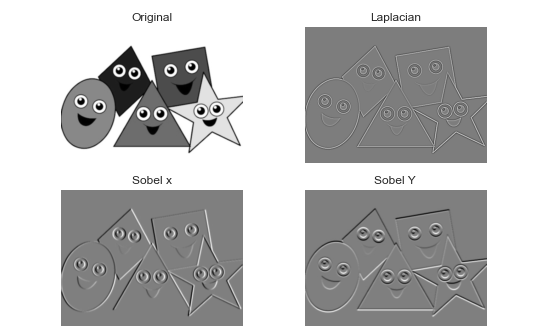
b) Edge detection schemes - the gradient (Sobel - first order derivatives)
based edge detector and the Laplacian (2nd order derivative, so it is
extremely sensitive to noise) based edge detector.

#Laplacian and Sobel Edge detecting methods
import cv2
import numpy as np
from matplotlib import pyplot as plt
#Loading image
#img0 = cv2.imread('SanFrancisco.jpg',)
img0= cv2.imread('Image.png',)
#converting to gray scale
gray = cv2.cvtColor(img0, cv2.COLOR_BGR2GRAY)
#remove noise
img= cv2.GaussianBlur (gray, (3,3),0)
#convolute with proper kernels
laplacian= cv2.Laplacian (img, cv2.CV_64F)
sobelx = cv2.Sobel(img,cv2.CV_64F,1,0,ksize=5) # x
sobely = cv2.Sobel(img,cv2.CV_64F,0,1,ksize=5) #y
plt.subplot(2,2,1), plt.imshow(img, cmap = 'gray')
plt.title('Original'), plt.xticks([]), plt.yticks([])
plt.subplot(2,2,2), plt.imshow(laplacian,cmap = 'gray')
plt.title('Laplacian'), plt.xticks([]), plt.yticks([])
plt.subplot(2,2,3), plt.imshow(sobelx, cmap = 'gray')
plt.title('Sobel x'), plt.xticks([]), plt.yticks([])
plt.subplot(2,2,4), plt.imshow(sobely,cmap = 'gray')
plt.title('Sobel Y'), plt.xticks([]), plt.yticks([])
plt.show()
OUTPUT

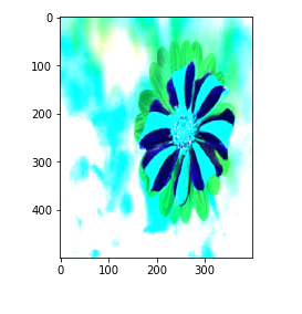
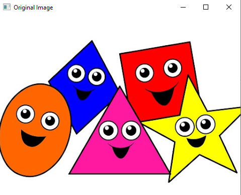
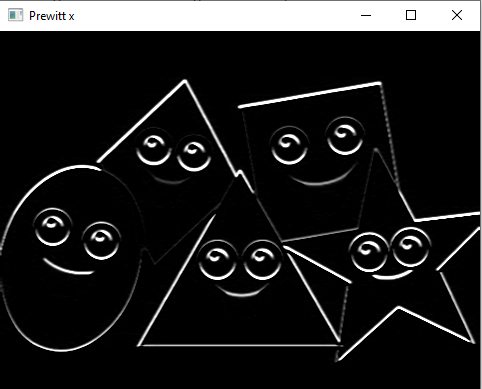
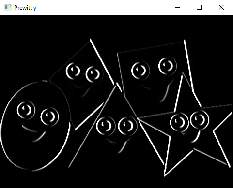
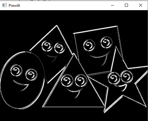
c) Edge detection using Prewitt Operator
#Edge detection using Prewitt operator
import cv2
import numpy as np
from matplotlib import pyplot as plt
img= cv2.imread('Image.png')
gray= cv2.cvtColor(img, cv2.COLOR_BGR2GRAY)
img_gaussian = cv2.GaussianBlur (gray, (3,3),0)
#prewitt
kernelx = np.array([[1,1,1],[0,0,0],[-1,-1,-1]])
kernely = np.array([[-1,0,1],[-1,0,1],[-1,0,1]])
img_prewittx= cv2.filter2D(img_gaussian, -1, kernelx)
img_prewitty = cv2.filter2D(img_gaussian, -1, kernely)
cv2.imshow("Original Image", img)
cv2.imshow("Prewitt x", img_prewittx)
cv2.imshow("Prewitt y", img_prewitty)
cv2.imshow("Prewitt", img_prewittx + img_prewitty)
cv2.waitKey()
cv2.destroyAllWindows()

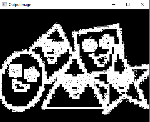
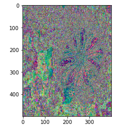
#Roberts Edge Detection- Roberts cross operator
import cv2
import numpy as np
from scipy import ndimage
from matplotlib import pyplot as plt
roberts_cross_v = np.array([[1,0],
[0,-1]])
roberts_cross_h = np.array([[0, 1],
[-1,0]])
img = cv2.imread("Image.png",0).astype('float64')
img/=255.0
vertical = ndimage.convolve(img, roberts_cross_v )
horizontal = ndimage.convolve( img, roberts_cross_h)
edged_img = np.sqrt( np.square (horizontal) + np.square(vertical))
edged_img*=255
cv2.imwrite("output.jpg",edged_img)
cv2.imshow("OutputImage", edged_img)
cv2.waitKey()
cv2.destroyAllwindows()

OUTPUT: