Local Sample Cohesion Normalization (LSCN)

LSCN is a normalization method designed for metabolomics data to correct for unwanted sample concentration or dilution effects while preserving inherent biological heterogeneity. Unlike conventional global normalization methods (e.g., CSN, L2N, PQN, Quantile Normalization), which rely on a single global reference and may obscure true biological variation, LSCN performs sample-specific normalization within local neighborhoods. It constructs a neighbor set for each sample in a reduced-dimensional space based on pairwise similarity and applies locally weighted normalization within these neighborhoods. This approach effectively removes technical bias without imposing artificial global uniformity. Developer is Fanjing Guo from Xiamen University of China.

Workflow of LSCN

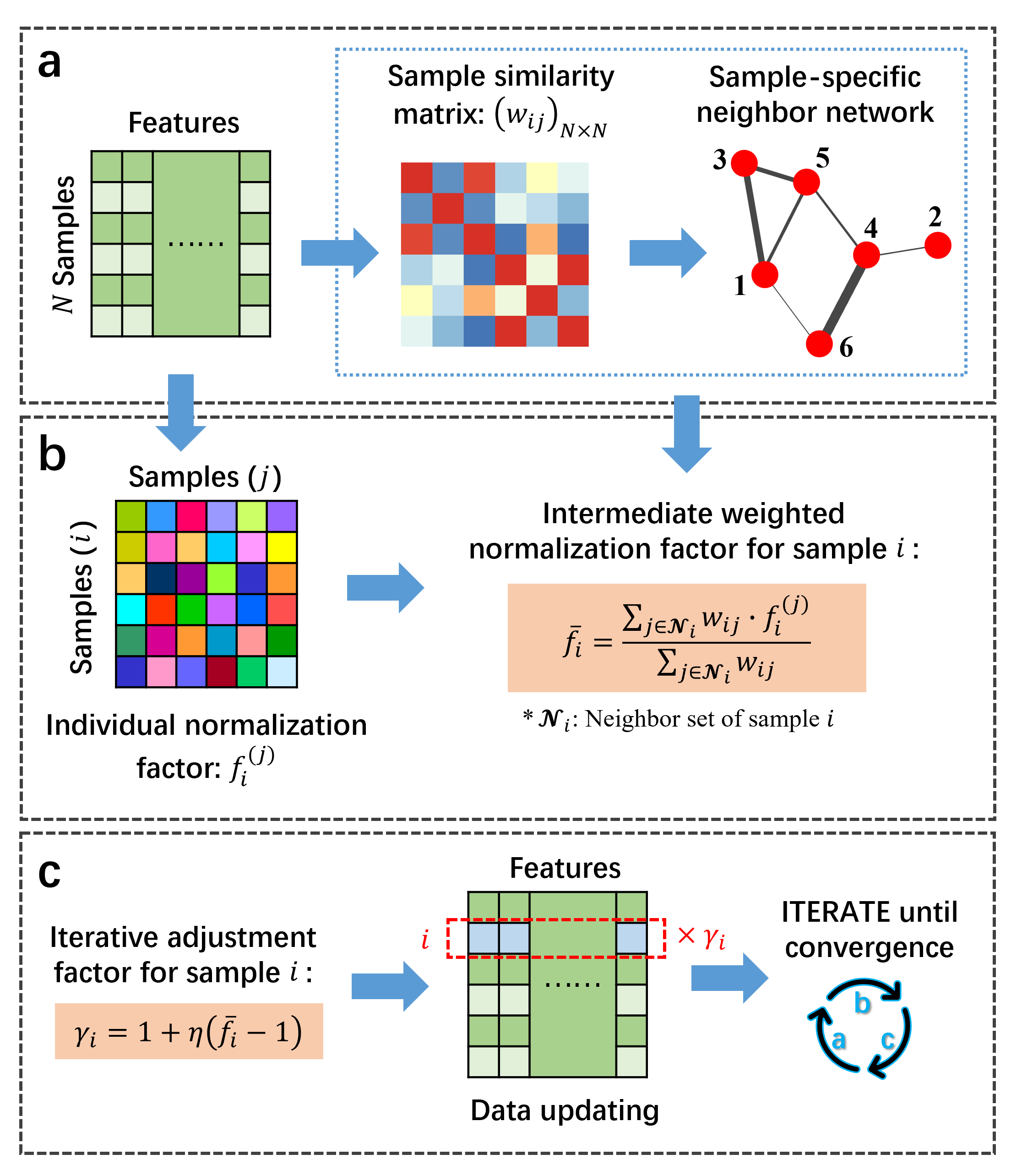
The workflow of LSCN algorithm. (a) Sample-specific neighbor set determination by constructing a neighbor network. (b) Intermediate weighted normalization factor calculation. (c) Data updating and iteration.

Requirement

R Environment

R version >= 4.4.0

Required Packages

The following R packages are essential for

the execution of the LSCN algorithm: philentropy, mixOmics, igraph, fpc, rlang.
the generation of a simulated dataset: mixOmics.
the evaluation on both simulated datasets and real biological datasets: all of the above packages and preprocessCore, ropls, networkD3, Rgraphviz, RBGL, MASS, car, factoextra, cluster, e1071, pROC, ggsci, colorspace, ggstar, ggraph, ggplot2, ggExtra, ggforce, caret, MLmetrics, progress, VennDiagram, nlme, DMwR2, energy, ROCR, here, tidygraph, patchwork, ggbreak, ggradar.

Installation Instructions

To install these packages, you can use the following R commands:

install.packages("philentropy")
install.packages("igraph")
install.packages("fpc")
install.packages("rlang")
install.packages("networkD3")
install.packages("MASS")
install.packages("car")
install.packages("factoextra")
install.packages("cluster")
install.packages("e1071")
install.packages("pROC")
install.packages("ggsci")
install.packages("colorspace")
install.packages("ggstar")
install.packages("ggraph")
install.packages("ggplot2")
install.packages("ggExtra")
install.packages("ggforce")
install.packages("caret")
install.packages("MLmetrics")
install.packages("progress")
install.packages("VennDiagram")
install.packages("nlme")
install.packages("energy")
install.packages("ROCR")
install.packages("here")
install.packages("tidygraph")
install.packages("patchwork")
install.packages("ggbreak")

if (!require("BiocManager", quietly = TRUE))
    install.packages("BiocManager")
BiocManager::install("mixOmics")
BiocManager::install("preprocessCore")
BiocManager::install("ropls")
BiocManager::install("Rgraphviz")
BiocManager::install("RBGL")
BiocManager::install("DMwR2")
BiocManager::install("ggradar")

Quickly Start

Normalization using LSCN

LSCN Function

LSCN(X, doLog = TRUE, k = NA, corr.thresh = NA, similar.type = 'WRA',
     simi.quant = NA, ita0 = 0.4, adjust_freq = 5,
     decayRate = 0.8, incRate = 1.1, max_ite = 100,
     eps = 1e-4, print.txt = FALSE)

Inputs

X: A data matrix with samples in rows and features in columns.
doLog: Logical, whether the data should be log-transformed. Default is TRUE.
k: Integer, the number of contaminated features. If NA, k = 0.05 * nrow(X).
corr.thresh: Positive real, the sample PCC cut-off threshold. If NA, an adaptive selection strategy will be used.
similar.type: One of ('CN', 'JC', 'SI', 'WPA', 'WAA', 'WRA'). Specifies the method used to estimate sample similarity. Default is 'WRA'.
simi.quant: A probability value which determines the sample similarity threshold. If NA, an adaptive selection strategy will be used.
ita0: A numeric value in the range (0, 0.5], the analogous learning rate. Default is 0.4.
adjust_freq: Integer, the number of iterations between each dynamic adjustment of the analogous learning rate. Default is 5.
decayRate: A numeric value between 0 and 1, the decay rate employed in the dynamic adjustment process of the analogous learning rate. Default is 0.8.
incRate: A numeric value larger than 1, the increase rate employed in the dynamic adjustment process of the analogous learning rate. Default is 1.1.
max_ite: Integer, the maximum number of iterations. Default is 100.
eps: Positive real, the convergence tolerance. Default is 1e-4.
print.txt: Logical, whether to print progress messages. Default is FALSE.

Outputs

dat.norm: The final normalized data matrix.
NORM.COEF: The normalization factors applied to the original data.
conv.vals: The recorded convergence criterion value in each iteration.
ita_history: The used analogous learning rate in each iteration.
RunTime: The run time of the function.

Step-by-Step Tutorial (LSCN)

Step 1: Install Required Packages Before using the LSCN function, ensure you have the necessary R packages installed. You can install them using the following commands:

install.packages("philentropy")
install.packages("igraph")
install.packages("fpc")
install.packages("rlang")

if (!require("BiocManager", quietly = TRUE))
    install.packages("BiocManager")
BiocManager::install("mixOmics")

Step 2: Load the LSCN implementation

source("Funcs_LSCN_Algorithm.R")

Step 3: Prepare Your Data Matrix Ensure your data is in the correct format or use the exemplary dataset:

data <- read.csv("example_dataset1.csv", header = T)

Step 4: Call the LSCN Function Call the LSCN function with your data matrix and desired parameters. For example:

Norm.Result <- LSCN(data, ita0 = 0.4, max_ite = 50, print.txt = T)
data.normalized <- Norm.Result$dat.norm
norm.factor <- Norm.Result$NORM.COEF
conv <- Norm.Result$conv.vals
runtime <- Norm.Result$RunTime

Step 5: Inspect the Results You can inspect the normalized data and other outputs as follows:

# View the normalized data matrix
View(data.normalized)

# View the normalization factors
print(norm.factor)

# Plot the convergence curve
library(ggplot2)
conv.df <- data.frame(iteration = c(1: length(conv)), 
                      value = conv)

ggplot(conv.df) + geom_line(aes(x = iteration, y = value)) + 
  geom_point(aes(x = iteration, y = value), shape = 21) + 
  theme_bw() + 
  xlab('Iteration') + 
  ylab('Value') + 
  theme(axis.title = element_text(size = 25, family = 'sans', face = 'bold'), 
        axis.text = element_text(size = 22, family = 'sans', face = "bold", color = 'black'), 
        legend.position = 'none', 
        panel.border = element_rect(linewidth = 2), 
        panel.grid = element_blank())

# Print the run time
print(runtime)

Generation of Simulated Datasets

Function

GenSimuDat(X, N = 100, selsamp.ratio = 0.9, 
           indiv.sd.ratio = 0.25, grpVar.ratio = 0.3, 
           grpEff.lamda = c(1, 3), grpEff.sd.ratio = 0.2, 
           subgrpNum = 3, topPC.num = 10, 
           diltF.m = 10, diltF.sd = 3, print.txt = F)

Inputs

X: Sample-by-feature data matrix that serves as the source of the base spectra.
N: Integer, the sample size of the simulated dataset. Default is 100.
selsamp.ratio: A probability value, the proportion of samples drawn from X to form a base spectrum. Default is 0.9.
indiv.sd.ratio: A numeric value between 0 and 1, the ratio of the standard deviation of individual differences to the mean feature intensity. Default is 0.25.
grpVar.ratio: A numeric value between 0 and 1, the proportion of randomly selected features with inter-group differences. Default is 0.3.
grpEff.lamda: A numeric vector with two elements, which determines the range of the inter-group difference magnitudes. Default is c(1, 3).
grpEff.sd.ratio: A numeric value between 0 and 1, which also determines the range of the inter-group difference magnitudes. Default is 0.3.
subgrpNum: Integer, the number of sub-groups. Default is 3.
topPC.num: Integer, the number of principal components to add intra-group heterogeneity. Default is 10.
diltF.m: A positive real value determines the distribution of dilution coefficients. Default is 10.
diltF.sd: A positive real value also determines the distribution of dilution coefficients. Default is 3.
print.txt: Logical, whether to print progress messages. Default is FALSE.

Outputs

BaseDat: The matrix of simulated base data.
IndivDat: The simulated data matrix after adding individual differences.
GrpDat: The simulated data matrix after adding individual differences and inter-group differences.
HeterDat: The simulated data matrix after adding individual differences, inter-group differences and intra-group heterogeneity.
SimuDat: The simulated data matrix after adding individual differences, inter-group differences, intra-group heterogeneity and dilution effects.
InitDat: The simulated data matrix before adding dilution effects.
Para: A list containing six elements: -- Ei: The matrix of the added individual differences; -- era.peak.ratio: The ratio of signals that are masked by individual differences; -- group: The simulated group label; -- DEmetIdx: The indices of the selected inter-group differential features; -- grpEff: The matrix of the added inter-group differences; -- diltF: The dilution coefficients.

Step-by-Step Tutorial (Generation of Simulated Datasets)

Step 1: Install Required Packages

if (!require("BiocManager", quietly = TRUE))
    install.packages("BiocManager")
BiocManager::install("mixOmics")

Step 2: Load the Function Implementation

source("Funcs_simulation.R")

Step 3: Prepare Your Data Matrix Ensure your data to generate simulated datasets is in the correct format or use the exemplary dataset:

data <- read.csv("example_dataset2.csv", header = T)

Step 4: Call the Function Call the associated function with your data matrix and desired parameters. For example:

# Generate a simualted dataset with default settings
Simu.Result <- GenSimuDat(data)
data.simulated <- Simu.Result$SimuDat

# Control the magnitude of individual differences 
Simu.Result <- GenSimuDat(data, indiv.sd.ratio = 0.05) # small
Simu.Result <- GenSimuDat(data, indiv.sd.ratio = 0.65) # large
data.simulated <- Simu.Result$SimuDat
indivdiff.mat <- Simu.Result$Para$Ei

# Control the magnitude of inter-group differences 
Simu.Result <- GenSimuDat(data, grpEff.lamda = c(0.3, 1)) # small
Simu.Result <- GenSimuDat(data, grpEff.lamda = c(10, 30)) # large
data.simulated <- Simu.Result$SimuDat
simu.group <- Simu.Result$Para$group
groupdiff.mat <- Simu.Result$Para$grpEff

# Control the number of inter-group differential features 
Simu.Result <- GenSimuDat(data, grpVar.ratio = 0.1) # small
Simu.Result <- GenSimuDat(data, grpVar.ratio = 0.7) # large
data.simulated <- Simu.Result$SimuDat
DE.Idx <- Simu.Result$Para$DEmetIdx # indices of differential features

# Control the number of sub-groups 
Simu.Result <- GenSimuDat(data, subgrpNum = 2) # small
Simu.Result <- GenSimuDat(data, subgrpNum = 10) # large
data.simulated <- Simu.Result$SimuDat

# Control the magnitude of dilution effects 
Simu.Result <- GenSimuDat(data, diltF.m = 1, diltF.sd = 0.1) # small
Simu.Result <- GenSimuDat(data, diltF.m = 100, diltF.sd = 30) # large
data.simulated <- Simu.Result$SimuDat
dilt.factor <- Simu.Result$Para$diltF

Step 5: Inspect the Results You can inspect the simulated data and other outputs as follows:

# View the simulated data matrix
View(data.simulated)

# View the added individual differences
View(indivdiff.mat)

# View the simulated group labels
print(simu.group)

# View the added inter-group differences
View(groupdiff.mat)

# View the indices of differential features
print(DE.Idx)

# View the dilution coefficients
print(dilt.factor)

Contact

Please contact me if you have any help: fjguo@stu.xmu.edu.cn

Name		Name	Last commit message	Last commit date
Latest commit History 9 Commits
Data		Data
Evaluation_Scripts		Evaluation_Scripts
LSCN_Function		LSCN_Function
Simulation_Code		Simulation_Code
LSCN_Workflow.png		LSCN_Workflow.png
Local Sample Cohesion Normalization.Rproj		Local Sample Cohesion Normalization.Rproj
README.md		README.md
example.R		example.R
example_dataset1.csv		example_dataset1.csv
example_dataset2.csv		example_dataset2.csv
lSCN_Workflow.png		lSCN_Workflow.png

Provide feedback

Saved searches

Use saved searches to filter your results more quickly

Repository files navigation

Local Sample Cohesion Normalization (LSCN)

Workflow of LSCN

Requirement

R Environment

Required Packages

Installation Instructions

Quickly Start

Normalization using LSCN

LSCN Function

Step-by-Step Tutorial (LSCN)

Generation of Simulated Datasets

Function

Step-by-Step Tutorial (Generation of Simulated Datasets)

Contact

About

Uh oh!

Releases

Packages

Uh oh!

Contributors

Uh oh!

Languages

Folders and files

Latest commit

History

Repository files navigation

Local Sample Cohesion Normalization (LSCN)

Workflow of LSCN

Requirement

R Environment

Required Packages

Installation Instructions

Quickly Start

Normalization using LSCN

LSCN Function

Step-by-Step Tutorial (LSCN)

Generation of Simulated Datasets

Function

Step-by-Step Tutorial (Generation of Simulated Datasets)

Contact

About

Resources

Uh oh!

Stars

Watchers

Forks

Releases

Packages 0

Uh oh!

Contributors

Uh oh!

Languages

Packages