Meeting Minutes

March XX, 2024

LnL nans

Likelihood equation: $$\log L(D|\lambda) = \log L_{\rm Poisson}(N_{obs}|\lambda) + \sum^{N_{obs}} \log p(D_i | \lambda)$$

Poisson LnL: $$\log L_{\rm Poisson}(N_{obs}|\lambda) \propto N_{obs} \log(N_{model}(\lambda))-N_{model}(\lambda)$$

(Note -- we ignore terms that depend on the data only. These disappear on normalisation, such as log(Nobs!) and permutation coefficients.)

Grid LnL: $$p(D_i | \lambda) = p(z=z_i, M_c=M_c,i|\lambda)$$

My bug was in the Grid LnL --> Im getting Nans when using ~1000 BBHs and even ~10 BBHs:

(aSF=0.01, dSF=4.70, mu_z=-0.01, sigma0=0.0)

Priors

    muz=[-0.5, -0.001],  # Jeff's alpha
    sigma0=[0.1, 0.6],  # Jeff's sigma
    aSF=[0.005, 0.015],
    dSF=[4.2, 5.2],

To reproduce nan:

    lnl, unc = McZGrid.lnl(
        mcz_obs=mock_data.observations.mcz,
        duration=1,
        compas_h5_path=mock_data.compas_filename,
        sf_sample=dict(aSF=0.01, dSF=4.70, mu_z=-0.01, sigma0=0.0),
        n_bootstraps=0,
        save_plots=True,
        outdir=f"{tmp_path}/nan_lnl"
    )

Code for section with Nan:

def ln_poisson_likelihood(
    n_obs: int, n_model: int, ignore_factorial=True
) -> float:
    """
    Computes LnL(N_obs | N_model) = N_obs * ln(N_model) - N_model - ln(N_obs!)

    :param n_obs: number of observed events
    :param n_model: number of events predicted by the model
    :param ignore_factorial: ignore the factorial term in the likelihood

    # TODO: Why are we ignoring the factorial term?? It was in Ilya's notes from 2023, but unsure why...

    :return: the log likelihood
    """
    if n_model <= 0:
        return -np.inf
    lnl = n_obs * np.log(n_model) - n_model

    if ignore_factorial is False:
        lnl += -np.log(np.math.factorial(n_obs))

    return lnl






def ln_mcz_grid_likelihood(
    mcz_obs: np.ndarray, model_prob_func: Callable
) -> float:
    """
    Computes LnL(mc, z | model) = sum_i  ln p(mc_i, z_i | model)     (for N_obs events)
    :param mcz_obs: [[mc,z], [mc,z], ...] Array of observed mc and z values for each event (exact measurement)
    :param model_prob_func: model_func(mc,z) -> prob(mc_i, z_i | model)
    :return:
    """
    return np.sum([np.log(model_prob_func(mc, z)) for mc, z in mcz_obs])


...


    def prob_of_mcz(self, mc: float, z: float, duration: float = 1.0) -> float:
        mc_bin, z_bin = self.get_matrix_bin_idx(mc, z)
        return self.rate_matrix[mc_bin, z_bin] / self.n_detections(duration)




# FINALLY: 
lnl = poisson_lnl + mcz_lnl

The self.n_detections(duration)--> 0 leading to the nan

is my Current fix valid: prob_of_mcz--> 0 if $N_{model}==0$?

Multimodal 1d Gaussian

Basic test

Posterior generation

PP-Plot

Feb 19th, 2024

Meeting with Jeff, Ilya, Chayan, Avi

Todos:

• Multimodal lnl distribution -- one bigger, one smaller peak (start at smaller peak), see if the different acquisition functions reach the higher peak (sharper peak but wider).

• difference between current and Maximum lnl off all points sampled (don't know ground truth, but we do know max LnL amongst all points)

• everything relative to MaxLnL

• LnL Nans: maybe because of small numbers --> Maybe I have lots of observations -- fewer detections will help avoid the nans -- right now we are using N-bbh = 1K, will this get fixed temporarily with N-bbh = 10s?

• Test generation of Posteriors (with 1D multimodal thing)

  • Use MCMC + surrogate LnL
    • When using uncertainty: If LnL: 25 +/- 2 (then we draw LnL from Norm(25, sigma=2))
    • When not using uncertainty: just take the surrogate Mean
  • compare analytical with surrogate posterior
  • make a PP-plot,

• Diagnostic plot:

  • When we have analytical: KL div between true posterior (analytical) + surrogate Posterior
  • For COMPAS: KL div between best posterior (ie after 10000 iterations) + current posterior

Summary

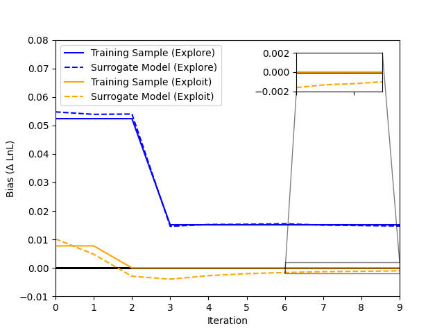
• Example of 'minimum' LnL training points and model predictions over iterations

• 1D sf example The 'errors' are much larger... hmm

• 2D sf example... sorry, forgot to include model predictions!

Params are aSF, dSF

Questions:

• Posterior from LnL -- do I need to sample, or just LnL * prior?
• using ilya's analytical Unc -- checked with group, for now this is OK (for production we'll need to move to bootstrapping)
• stopping criteria for BayesOpt?

Jan 31st, 2024

Meeting with Jeff, Ilya, Chayan, Avi

NExt steps:

• Assume COMPAS run producing the 'correct' universe
• making regret plot with both surrogate and tru LnL
• can we zoom into main region -- meaningful posteriors?

different threads for this project:

1. how good of a LnL estimate do we need? What is the correct tradeoff between making COMPAS calls (1000 points in parameter space with high fidelity), and surrogate modeling
2. Best way to create an acquisition function?

Jeff: How do we choose best 'x' for acquisition -- can we use covarience

Avi: Do we really need a LnL surrogate or more just an active learning method to find 'interesting' regions of parameter space?

Ilya:

• I think we ultimately want to zoom in, a lot. A difference of even 100 in ln likelihood, which is about the most I can resolve on this plot, means these parameters are 10^{43} times more/less likely -- that's huge, and would mean the parameters in question are far outside any credible interval of interest.

• Are lnL NANs because you are multiplying / dividing by numbers that are too large / small? Sometimes it's a question of offsetting things relative to some suitable fixed value rather than computing absolute likelihoods.

Ilya's notes on LnL uncertainty:

What is the expected level of fluctuation in the log likelihood due to statistical sampling errors?
We can think of the likelihood as a product of likelihoods of the observed count of events c_i given Poisson predictions n_i for the count of events in each bin i in Mchirp-redshift space.  Thus, the log likelihood is the sum of log likelihoods over each bin.  The Poisson likelihood in each bin is

L_i = exp(-n_i) n_i^c_i / c_i!

Ignoring the denominator (which depends only on data, and is thus a normalisation constant),
log L_i = -n_i + c_i log n_i.

Then the total log likelihood is
log L = - \sum_i n_i + \sum_i c_i log n_i.

Suppose there is an error d_i in the predicted counts in each bin due to sampling uncertainties.  Assume d_i << n_i; then
log (n_i+d_i) = log(n_i) log(1+d_i/n_i) ~ log(n_i) (1+ d_i/n_i - (1/2) (d_i/n_i)^2 + ...).

The associated error in log L will then be
d log L ~ - \sum_i d_i + \sum_i c_i (d_i/n_i) log n_i + ... = - \sum_i d_i + \sum_i d_i (c_i/n_i) log n_i + ...

The first term is easy: it's just the fluctuation in the total number of expected detections due to finite sampling accuracy.
For a given i, the second term can generally be larger than the first term, i.e., (c_i/n_i) log n_i can be larger than 1.  However, the total contribution of the first term will generally be of the same order or greater than the second term, because of the stochastic nature of the second term (the number of observations in some bins exceeds expectations while there are too few observations in other bins).
To see this, let's include some assumptions which aren't necessary but which will simplify the argument, and consider two extreme regimes.  The additional assumptions are that d_i and n_i are the same in all K bins, i.e., n_i=N/K and d_i = D/K. Let's further suppose we are evaluating the likelihood at the true model parameters, so that all c_i are independently drawn from a Poisson distribution with expectation value N/K.   The two regimes we will consider are (a) n_i = N/K ~ a few and (b) n_i = N/K \ll 1.  In both regimes, the first term sums up to D.

In regime (a), we expect that c_i have a scatter of \sqrt{N/K} around the expectation value of N/K.  Typically, sqrt(K) of the elements in the second term will be too large (or too small). The second term will then have a typical value of sqrt(K) (D/K) log(N/K).   Thus, the second term is of order the first term times log(N/K) / sqrt(K).  As long as the number of bins is sufficiently large that sqrt(K) > log(N/K), the first term dominates or sets the expected size of the fluctuation in log L.
In regime (b), we expect that the bins are sufficiently finely pixellated so that the number of expected detections in any one bin is small, n_i = N/K \ll 1.  Then, c_i should all be either zero or 1.  When they are zero, the pixels contribute nothing to the second term.  The total number of pixels we expect to contribute is ~N.  The second term is thus N ((D/K) / (N/K)) log (N/K) ~ D log(N/K).  While the second term can then be a factor of |log(N/K)| larger than the first term, this is only a logarithmic scaling.  Moreover, it is really the effective K (the number of pixels containing the majority of the expectation value) that should be used here.  Thus, as long as the effective K is not too many orders of magnitude larger than N, it's still safe to say that the fluctuation in log L from statistical sampling uncertainty is no more than a few times (log(N/Keff), to be precise) larger than the statistical uncertainty in the total number of expected detections.

Jan 10, 2024

Some notes on exploration strategies and acquisition functions

$x_{\rm next} = {\rm GetQuery}(model, data) = {\rm arg max} \alpha(x; model, data)$

Where is the next point that maximizes the future value of the model??

check out this lecture

Sample(model, x)	Thompson Sampling	Least likely to be stuck at locals, sample GP-posterior, maximumise sampled function
GetTail(model, x, threshold)	PI (probability of improvement)	Greedy -- local optima, not best for high dimensions, or multimodal distributions
GetImprovement(model, x, threshold)	EI (expected improvement)/EGO	Expectation instead of probability, considered more global than PI
GetQuantile(model, x, quantile)	UCB (upper confidence bound)	The acquisition function 'envelops' max uncertainty/quantile at a region
GetEntropy(model, x)	PES (predictive entropy search)

The acquisition function needs to be selected/configured to balance the following depending on your task:

• EXPLOIT: Maximize function f
• EXPLORE: "LEARN" function f

Paper that studies switching acquisition functions:

Check out PI is back! Switching Acquisition Functions in Bayesian Optimization

They switch between different acquisition functions -- what we want to do!

They use:

• EI -- explorative AF
• PI -- exploitative AF

And state:

if the properties of the problem to optimize are unknown, switching from EI to PI after 25 % of the budget of surrogate-based evaluations should be favored.

Related papers:

• Self-Adjusting Weighted Expected Improvement for Bayesian Optimization
• Mastering the exploration-exploitation trade-off in Bayesian Optimization

'Regret' plot

This is a 'regret' plot looking at different acquisition functions. The red line marks the LnL when using the 'true' parameters.

Dec 20, 2023

• Chayan, Jeff, Avi chat about project + bring Chayan up to speed
• Slides from COMPAS group meeting

Action items

• Add chayan to https://github.com/COMPAS-Surrogate (need Chayan's username etc)
• chayan to investigate TFprobability, etc as surrogate options
• Avi to make an example of the

Dec 15, 2023

• Avi's main progress Dec 12-14:

  • Refactor LnL computation
  • slurm utils for pipeline
  • faster acquisition function test cases (see this test)

• QUESTIONS:

  • Multiple dimension acquisition function?
  • Go over params to be used--> ["aSF", "dSF", "mu_z", "sigma_z"]??
    • https://www.praescientem.com.au/publications/Riley_2023_ApJ_950_80.pdf
    • it should be mu0 sigma0
  • Ask about using posteriors vs list of 'delta' functions of Mc-Z mock observations
  • Ilya's suggestion for faster bootstraps?
  • code design for acquisition functions for generalized models? Where should this code live?

• Remaining TODOs:

  • DNN model for [Sf params] --> [Lnl, unc] (output both)
  • testing out multi-D acquisition function...

Nov 2, 2023

Things to discuss:

• COMPAS surrogate results
• GP with uncertain inputs
• Acquisition function

Code overview

All repos here: https://github.com/COMPAS-Surrogate/

• LnL computer:

  • Generates training data (runs cosmic-int, saves matrices, computes LnL)
  • Generate matrices with make_detection_matricies --aSF 0.1 --dSf ...
  • Or make_detection_matricies --param_csv data.csv
  • After, compute_lnl --detection-matrices matrices.hdf --data universe.hdf
  • QS: Maybe just save LnL, don't bother saving matrices?
  • TODO: add in slurm generator

• LnL surrogate:

  • Contains surrogate models (GPFlow, SklearnGP, SklearnMLP, TfDNN)
  • Contains acquisition-functions (not working for more than 1D atm)

• Pipeline:

  • Will contain slurm pipeline builder for N repetitions of Compute + Surrogate + acquisition
  • Currently contains bunch of python manual testing workflows

COMPAS surrogate results

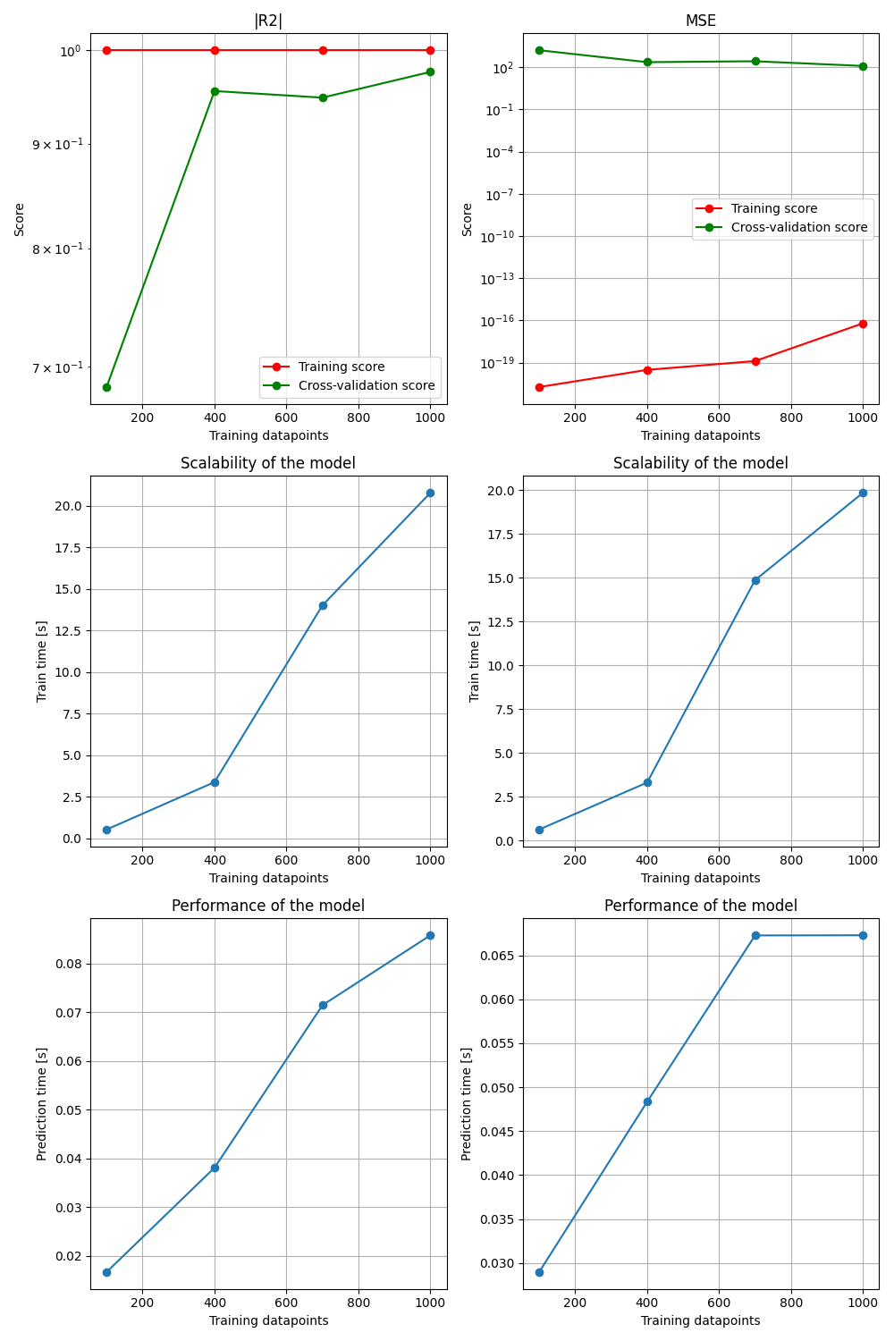
• Without incorporating LnL uncertainty, results "look" ok, but the validation error is high (overfitting)

• LnL + unc surrogate has a high training error (even with some random points)

• Something is going wrong in the GP surrogate model.

GP with uncertain inputs

Currently testing with GPFlow (a 'deep' GP) and sklearn.GP

• GPs perform well when not using uncertain inputs (LnL unc), and perform well in 1D (with uncertain inputs).
• GPs not performing well with 2+D with uncertain inputs...

QS

1. What about a DNN with two outputs (lnl + lnl unc) ?
2. What about bootstrapping the surrogate outputs (train N surrogates with different data, combine results + get LnL unc)
3. What about adding a "Noise" kernel to the GP? Do we expect the noise to be Gaussian? NO NEED FOR BOOTSTRAPS_??

Name	Image
gpflow_quadratic_uncFalse_n20
gpflow_quadratic_uncFalse_n50
gpflow_quadratic_uncTrue_n20
gpflow_quadratic_uncTrue_n50
sklearngp_quadratic_uncFalse_n10
sklearngp_quadratic_uncFalse_n20
sklearngp_quadratic_uncFalse_n50
sklearngp_quadratic_uncTrue_n10
sklearngp_quadratic_uncTrue_n20
sklearngp_quadratic_uncTrue_n50
gpflow_n10
gpflow_n25
gpflow_n50
sklearngp_n10
sklearngp_n25
sklearngp_n50

Acquisition functions:

Instead of coding our own, maybe we can leverage pre-existing BO tools? (note: some of these require a GP to be trained using an MCMC)

• https://modal-python.readthedocs.io/en/latest/content/examples/active_regression.html?highlight=regression%20multiple%20dimension#Active-regression

• https://gpax.readthedocs.io/en/latest/examples.html

• https://docs.jaxgaussianprocesses.com/examples/bayesian_optimisation/#a-more-challenging-example-the-six-hump-camel-function

Oct 3, 2023

Summary of project:

There are 4 parts to this project:

1. COMPAS-specific questions: how to compute likelihoods and uncertainties on them which arise because of how COMPAS computes those likelihoods, how large do simulations need to be in order to achieve sufficiently low uncertainties;

2. How to build surrogate models for the log-likelihood question over the COMPAS parameter space;

3. How to do active learning if we want to iteratively improve the log-likelihood surrogate model;

4. Using the surrogate model to infer the COMPAS parameters from LVK Data -- while that's sufficiently trivial with a good likelihood model in hand, there's a potential question of whether/how to incorporate the surrogate model uncertainty into posterior distributions on the parameters. However, let's leave that for now; simple version is to draw likelihoods for given parameters from the surrogate model including its uncertainty.

ILYA'S NOTES

Notes on uncertainty

On 1, Ilya did a crude analytical estimate that suggests that the COMPAS-sampling uncertainty in log-likelihood is of the order of the sampling uncertainty in the number of predicted events (detections), as long we are near max log-likelihood. Avi and Jeff will check that; if true, it should help us understand how many samples we'll need.

TAKEAWAY: Bootstraps are always relatively "cheap" because they don't require actual reruns of the full analysis (this will be particularly obvious when we go from varying post-processing MSSF parameters to varying COMPAS C++ model parameters). But, in general, the fractional accuracy of the bootstrap uncertainty estimate scales as 1/sqrt{N_boostraps}. So 100 bootstraps will give you a 10% fractional accuracy of the uncertainty in the quantity of interest due to finite sampling, which should indeed be good enough for our purposes.

Notes on surrogate

On 2, Avi tried a few things -- scikit-learn, GPflow, GPJax. We can use any off-the-shelf tool if it's good enough, doesn't need to be perfect. Avi seems to like GPJax, so that should be fine. By the way, I'd also suggest just using point estimates for the mean and standard deviation of the GP predictor for the log-likelihood at any location in the COMPAS parameter space (if doing inference on GP hyper-parameters, as GPJax does, can just pick MAP values).

Notes on acquisition

On 3, the question is really what is the best acquisition function. A proposal based on our conversations and some literature is to use the following:

75% of the time (can play with the fraction), use A = exp (-(mu - mu_max)^2/2 sigma^2), where mu and sigma are the mean and standard deviation of the GP predictor for log likelihood, and mu_max is its max value; 25% of the time, use A = sigma The idea is that most of the time, we are only interested in improving the surrogate model in places where the likelihood has a decent chance of being higher than the currently known maximum; but sometime, to avoid getting stuck, we just want to make more evaluations in places where the surrogate model is particularly uncertain.

Also, I'm thinking that we might want to think of (normalised) A as a probability distribution for drawing the next location for a COMPAS evaluation rather than just using the parameters where A is maximal, again to avoid getting stuck, and perhaps to better prepare for the situation when we'll want to draw the next 100 parameters for evaluation rather than going through 1 step at a time (more efficient in terms of wall time when we have 100 cores available). Though in that case, we really should think of how to penalise the cost function for proposed parameter space location x_{i+1} based on the new proposals x_1...x_i, which isn't accounted for here.

Sept 5, 2023

Number of DCOs from N Compas runs -- Poisson distributions.

Currently for bootstrapping

for n trials:
    n_dcos[I] = N original + Normal( sqrt(N))  

Illya's suggestion:

• We have 1 COMPAS run with 'k' DCOs.
• Draw x from Poisson(mean=k)

bootstrap_lnl_vals = zeros(n_bootstraps)

for i in n_bootstraps:
   n_dcos= Poisson(lambda=l).sample() 
   compas_seeds = original_compas_population_seeds.sample(n_dcos)
   bootstrap_lnl_vals[i] = likelihood(data, compas_seeds)

unc = std(lnl_vals)
lnl = likelihood(data, original_compas_seeds)

1. Tests with LnL unc Ilya predicts uncertainty in LnL ~ uncertainty in N detections. Uncertainty in LnL will increase with more detections.

Tests for increasing number of bootstraps

• simulate population
• get LnL + 1000 bootstrap Lnl
• see what the Std(bootstrap lnl) is for different number of bootstraps
• also store the number of detections for all bootstrap events

2. GPU LnL?

Aug 23, 2023

	D1	D2	D3
EI
TH
UCB
UE

`![dataset_1_ei](https://github.com/avivajpeyi/compas_ml_surrogate/assets/15642823/2cda4d1b-6cb0-4ce5-96b5-48d9cbf0790c)`
`![dataset_1_thompson](https://github.com/avivajpeyi/compas_ml_surrogate/assets/15642823/97bc210f-c29c-4b12-8c7f-a3bb8b5abd47)`
`![dataset_1_ucb](https://github.com/avivajpeyi/compas_ml_surrogate/assets/15642823/e1943785-7ea4-4079-99d3-29abb2041a1d)`
`![dataset_1_ue](https://github.com/avivajpeyi/compas_ml_surrogate/assets/15642823/9f6a16cb-0be3-4a0c-8472-53e30e3bcc63)`


`![dataset_2_ei](https://github.com/avivajpeyi/compas_ml_surrogate/assets/15642823/7ef729fc-8f95-40cb-b1a2-e1171eceec43)`
`![dataset_2_thompson](https://github.com/avivajpeyi/compas_ml_surrogate/assets/15642823/7e9a36a5-d4d6-4593-a9d3-2ce706ccb5dc)`
`![dataset_2_ucb](https://github.com/avivajpeyi/compas_ml_surrogate/assets/15642823/42e89e23-1e5b-44e0-a78b-259f52869c16)`
`![dataset_2_ue](https://github.com/avivajpeyi/compas_ml_surrogate/assets/15642823/bd35eded-89c0-4f5c-a080-04010230e463)`




`![dataset_3_ei](https://github.com/avivajpeyi/compas_ml_surrogate/assets/15642823/da7ad5b4-820b-4ce9-9680-1cf7cd50ed4f)`
`![dataset_3_thompson](https://github.com/avivajpeyi/compas_ml_surrogate/assets/15642823/aa33ad19-e249-44d8-b5ee-f628a12266a8)`
`![dataset_3_ucb](https://github.com/avivajpeyi/compas_ml_surrogate/assets/15642823/d6184215-0e05-4388-88bb-82228ea6b200)`
`![dataset_3_ue](https://github.com/avivajpeyi/compas_ml_surrogate/assets/15642823/2691afbf-76d5-4168-b6e5-d5a210f31a2e)`



![d1_goodqUCB](https://github.com/avivajpeyi/compas_ml_surrogate/assets/15642823/2be19245-50e4-482a-8979-e171ae33103b)
![d1_badqUCB](https://github.com/avivajpeyi/compas_ml_surrogate/assets/15642823/cb9a7e54-c71b-4d4d-8229-387f2f53450e)
![d1_mse](https://github.com/avivajpeyi/compas_ml_surrogate/assets/15642823/c1858c15-2219-40f5-975f-228e329f3f78)
![d2_mse](https://github.com/avivajpeyi/compas_ml_surrogate/assets/15642823/881896f6-42e4-4ab9-b56c-c69190a60443)
![d3_mse](https://github.com/avivajpeyi/compas_ml_surrogate/assets/15642823/58cb8d2c-315e-4276-ae2c-77a030655686)

Aug 13, 2023

Papers on Active learning

Methods/Algos

1. uncertainty-based sampling: least confident (Lewis and Catlett), max margin and max entropy
2. committee-based algorithms: vote entropy, consensus entropy and max disagreement (Cohn et al.)
3. multilabel strategies: SVM binary minimum (Brinker), max loss, mean max loss, (Li et al.) MinConfidence, MeanConfidence, MinScore, MeanScore (Esuli and Sebastiani)
4. expected error reduction: binary and log loss (Roy and McCallum)
5. Bayesian optimization: probability of improvement, expected improvement and upper confidence bound (Snoek et al.)
6. batch active learning: ranked batch-mode sampling (Cardoso et al.)
7. information density framework (McCallum and Nigam)
8. stream-based sampling (Atlas et al.)
9. active regression with max standard deviance sampling for Gaussian processes or ensemble regressors

How to estimate uncertainty in Deep Learning networks

• Excellent tutorial from AGW on Bayesian Deep Learning

• This tut is inspired by his publication Bayesian Deep Learning and a Probabilistic Perspective of Generalization

• Dropout as a Bayesian Approximation: Representing Model Uncertainty in Deep Learning (Gal and Ghahramani, 2016) This describes Monte-Carlo Dropout, a way to estimate uncertainty through stochastic dropout at test time

• Bayesian Uncertainty Estimation for Batch Normalized Deep Networks (Teye et al. 2018) This describes Monte-Carlo BatchNorm, a way to estimate uncertainty through random batch norm parameters at test time

• Bayesian Deep Learning and a Probabilistic Perspective of Generalization (Gordon Wilson and Izmailov, 2020) Presentation of multi-SWAG a mix between VI and Ensembles.

• Advances in Variational inference (Zhang et al, 2018) Gives a quick introduction to VI and the most recent advances.

• A Simple Baseline for Bayesian Uncertainty in Deep Learning (Maddox et al. 2019) Presents SWAG, an easy way to create ensembles.

Bayesian active learning

• Deep Bayesian Active Learning with Image Data (Gal and Islam and Ghahramani, 2017) Fundamental paper on how to do Bayesian active learning.

• Sampling bias in active learning (Dasgupta 2009) Presents sampling bias and how to solve it by combining heuristics and random selection.

• Bayesian Active Learning for Classification and Preference Learning (Houlsby et al. 2011) Fundamental paper on one of the main heuristic BALD.

GP and active learning

• Exploration of lattice Hamiltonians for functional and structural discovery via Gaussian process-based exploration–exploitation

• Active Learning for Deep Gaussian Process Surrogates

• Actively learning GP dynamics

General

• Review paper: https://arxiv.org/abs/2009.00236
• Book on Active learning: https://www.manning.com/books/human-in-the-loop-machine-learning
• "Towards Robust Deep Active Learning for Scientific Computing" https://arxiv.org/abs/2201.12632
• Deep bayesian active learning + image https://arxiv.org/abs/1703.02910
• A Comparative Survey of Deep Active Learning: https://arxiv.org/abs/2203.13450

Tutorials/worksops

• Google's Active Learning Playground: This is a python module for experimenting with different active learning algorithms.
• deep-active-learning: Python implementations of the following active learning algorithms
• PyTorch Active Learning: Library for common Active Learning methods
• active-learning-workshop:KDD 2018 Hands-on Tutorial: Active learning and transfer learning at scale with R and Python. PDF

Codebases

1. Modal

Built on scipy+sklearn https://github.com/modAL-python/modAL

2. gpax

Gaussian processes + active learning! Very new, uses JAX ❤️ + numpyro Problem: unstable/

https://github.com/ziatdinovmax/gpax/

3. Scikit-activeml

https://www.preprints.org/manuscript/202103.0194/v1 https://pypi.org/project/scikit-activeml/

Also built on scipy+sklearn

3. Baal

A " Bayesian active learning library" Built on pytorch Seems like focus on images https://baal.readthedocs.io/en/latest/notebooks/compatibility/sklearn_tutorial/ https://baal.readthedocs.io/en/latest/ https://arxiv.org/abs/2006.09916

4. DeepAL

https://github.com/ej0cl6/deep-active-learning

5. adaptive

Adaptive sampling technique for 'learning' functional representation of the data https://adaptive.readthedocs.io/en/latest/index.html https://github.com/python-adaptive/adaptive/tree/v1.0.0

6. AliPy Agnostic of pytorch/sklearn/tflow

https://github.com/NUAA-AL/alipy

7. libact Features the active learning by learning meta-strategy that allows the machine to automatically learn the best strategy on the fly.

Works with sklearn

Hasnt been updated in 2 years https://github.com/ntucllab/libact

May 12, 2023

1. LnL surface smooth Ilya helped me find a bug, Lnl surface now looks smooth! woohoo!

2. bootstrapped uncertainty

• generate additional COMPAS datasets* and compute LnL
• use different Lnl to estimate a mean + std (to use in the GP uncertainty)

3. some injections

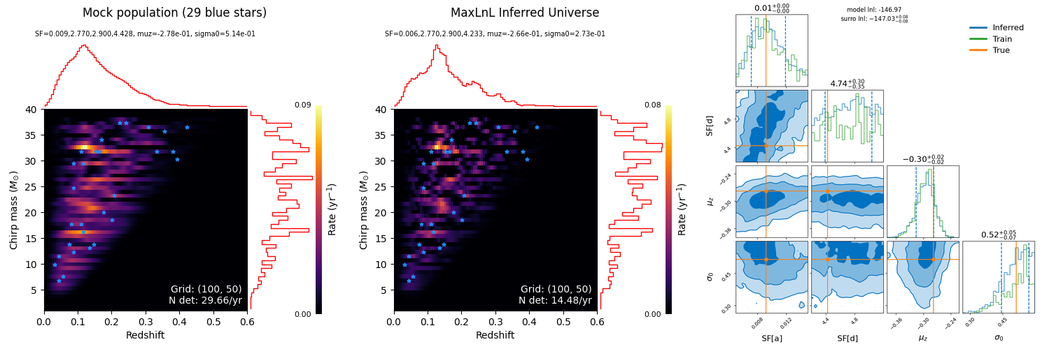
Percentile-percentile plot made using 50 sets of {aSF, dSF, mu0, sigma0} posteriors.

Posteriors were generated by running inference w/ nested sampling on 50 mock BBH catalogs with our sklearn-GP trained lnLikelihood(aSF, dSF, mu0, sigma0 | mock BBH catalog). The sklearn-GP was given 1600 training points (and a bootstrapped LnL uncertainty). I used very low sampler settings to get things running quickly (nlive=250,)

---

NExt steps

• relative unc in lnl -- record the number of merging binaries -- record total -- record number in mock datasets -- active learning -- latin hyper cube -- sequentially sample -- is deepGP better or sklearn better? -- some training plots using deepGP and sklearn gp

Paper thoughts

-- compare with Jeff's work -- does my active learning improve computational costs? -- does emulating LnL help rather than training ChirpM Z? Emulating one number rather than several hundred emulators

April 21, 2023

Plots of LnL Surface (muz, sigma0)

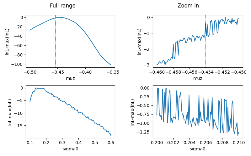
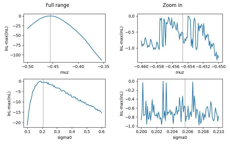
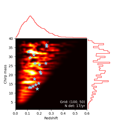
• Black dashed line -- true injection SF parameter value (used to generate detection matrix)
• Blue stars -- sampled events from the detection matrix

	2D	1D
Injection 1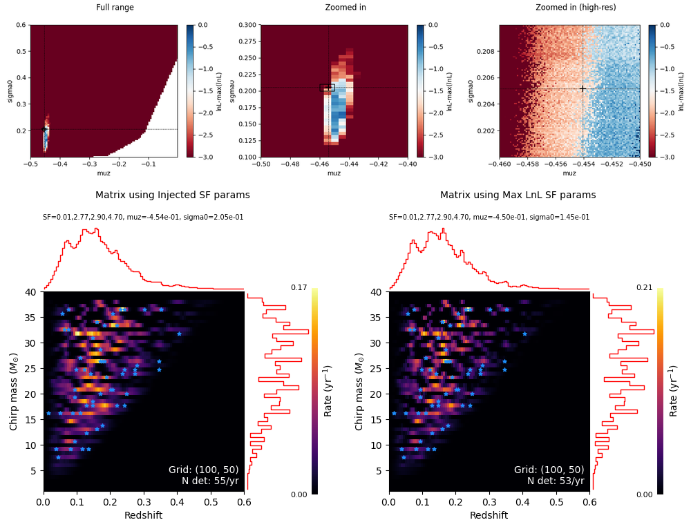
Injection 2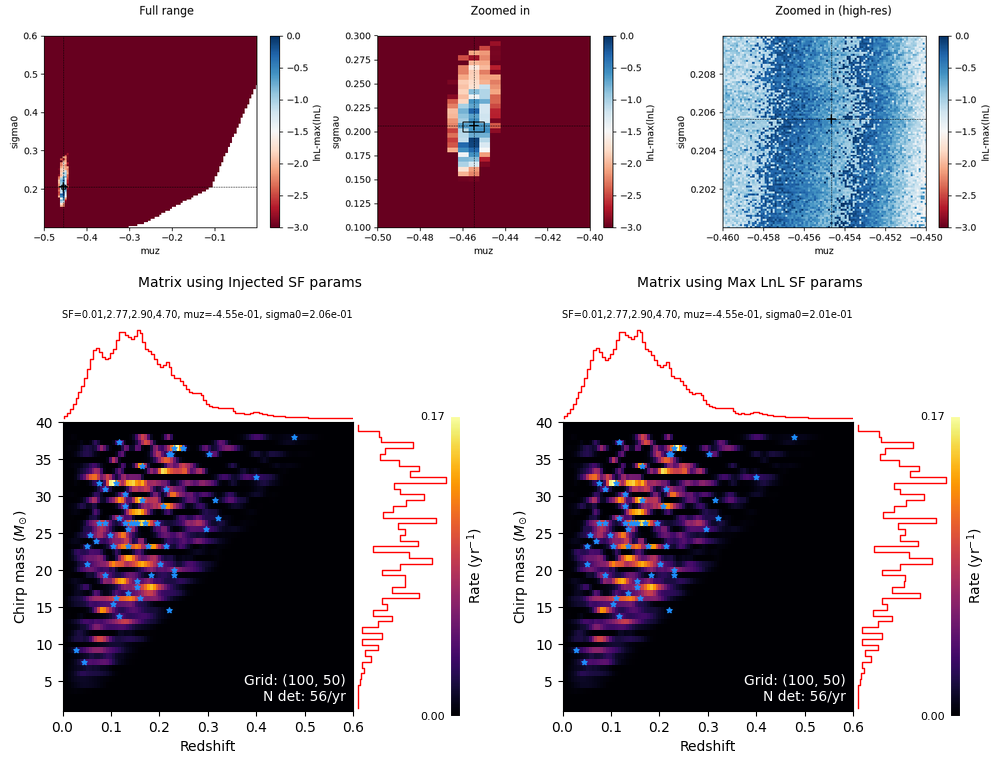

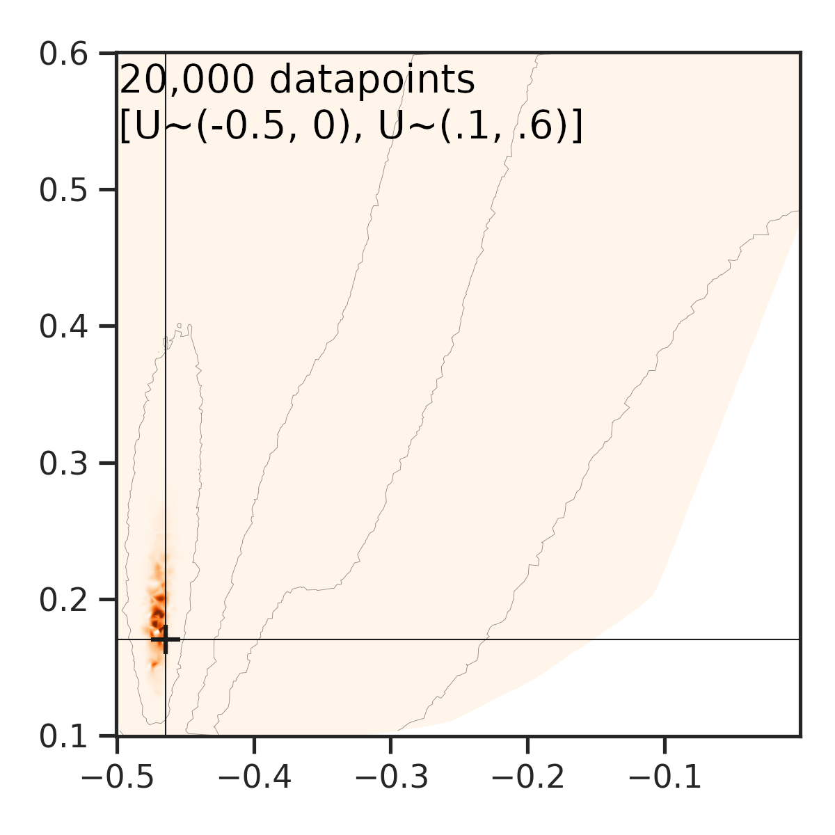
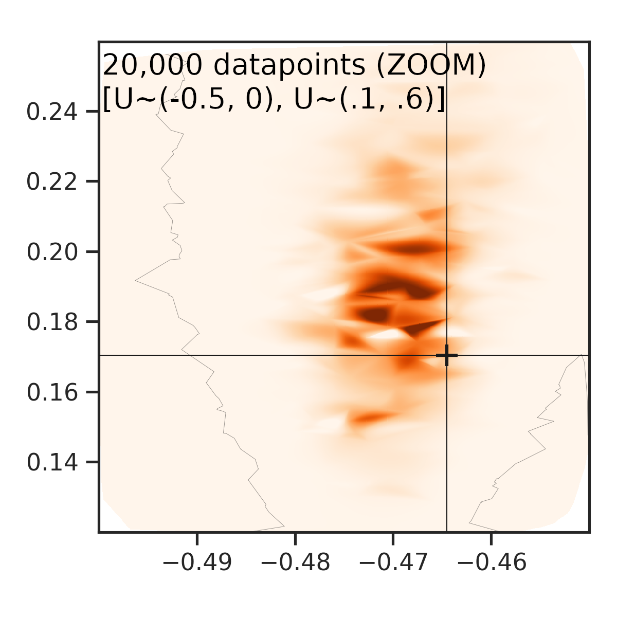
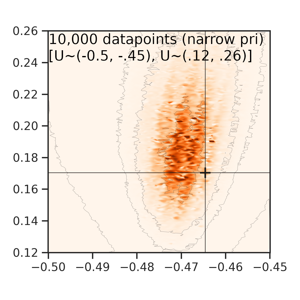
Some plots generated by:

• drawing random samples with prior-range
• computing likelihood and interpolating between points

Full parameter space	Zoom	More data points in zoomed area

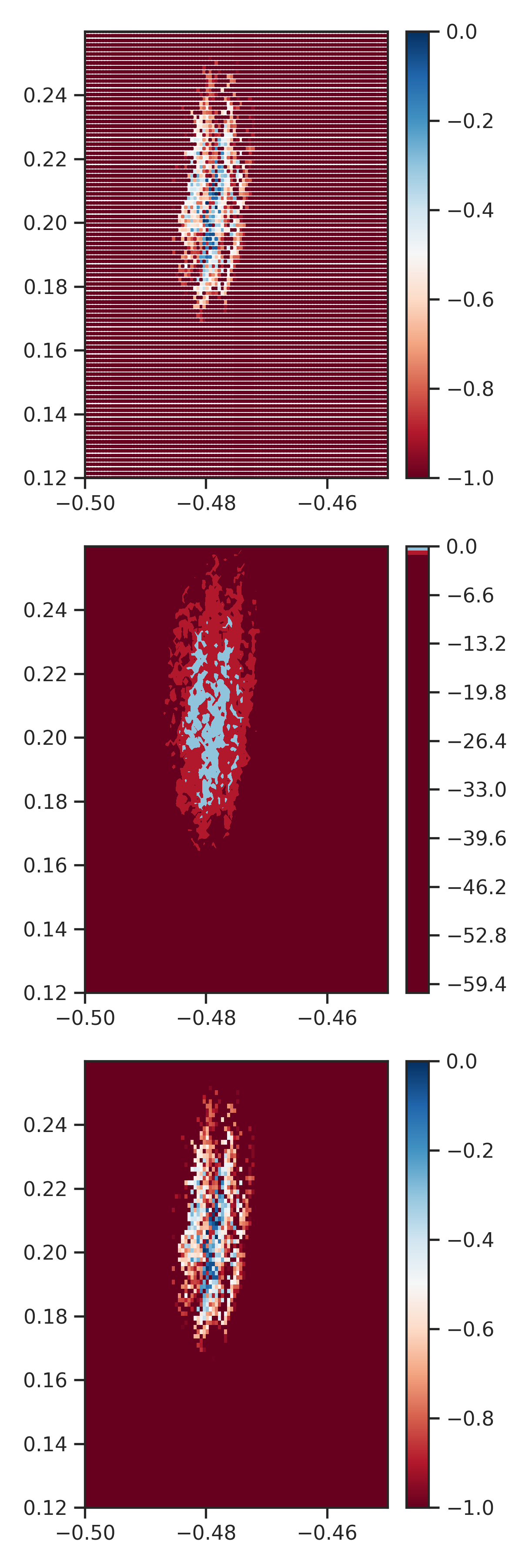
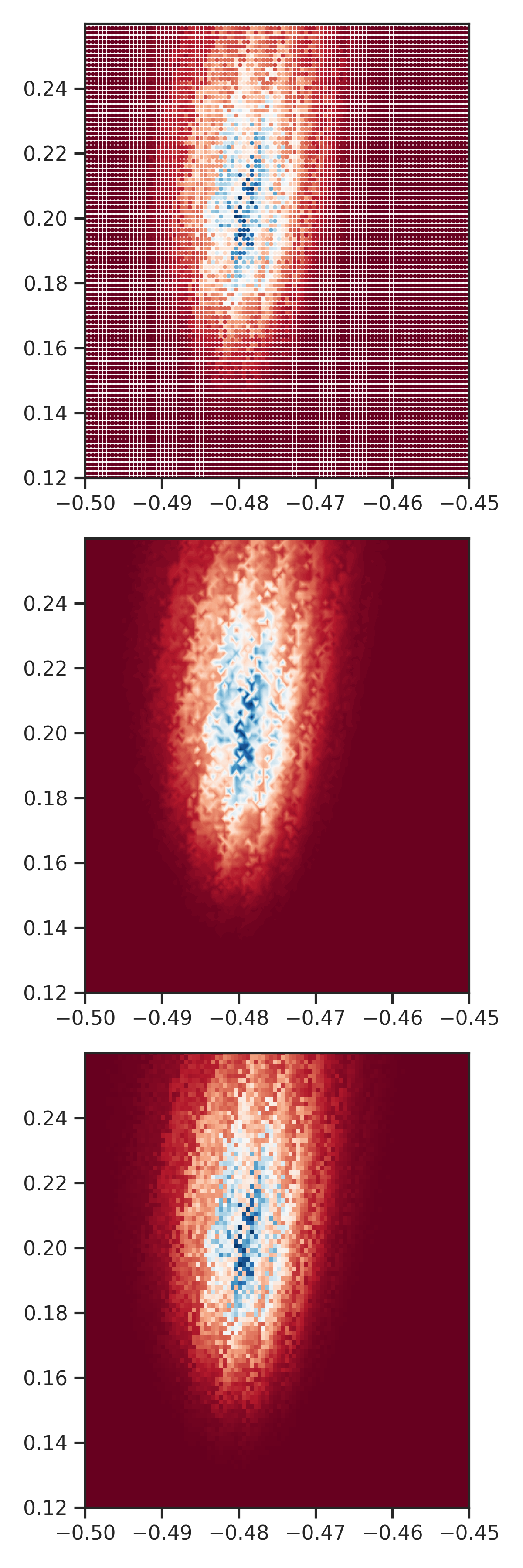
A different version of plot:

• linearly spaced grid of points
• top: scatter plot with likelihood values colored
• mid: interpolate between scatter plot points
• bot: imshow( log_likelihood - max(log_likelihood)) of data (no interpolation)
• limit color bar from 0 to -1

ln likelihood	likelihood

Zooming in further I am computing the likelihood and zooming in further -- this will take some time

BOOTSTRAP LnL uncertainty

• resample population with N + sqrt(N) (with replacements)
• compute list of LnL with different populations and obtain a boot-strapped LnL

Talk with Indranil

• LnL surface quite unsmooth, but just near the peak

1. Maybe try to figure about a hack to "smooth out" the likelihood
2. Need to ensure that training data is generated near the peak -- maybe something like 'subset simulation' to hone in on 'rare' events

https://www.researchgate.net/publication/320798357_A_short_report_on_PYTHON_implementation_of_subset_simulation https://onlinelibrary.wiley.com/doi/epdf/10.1002/jcc.24900 https://github.com/jpmit/lennyffs https://github.com/hackl/pyre https://archive.org/details/arxiv-1104.3667

March 11, 2023

Exploring the number of training points needed

Tried sampler after training with [10 - 10 000] data points (spaced by 100). The sampler failed (nburn > nsteps, with nsteps=1000).

n	image
100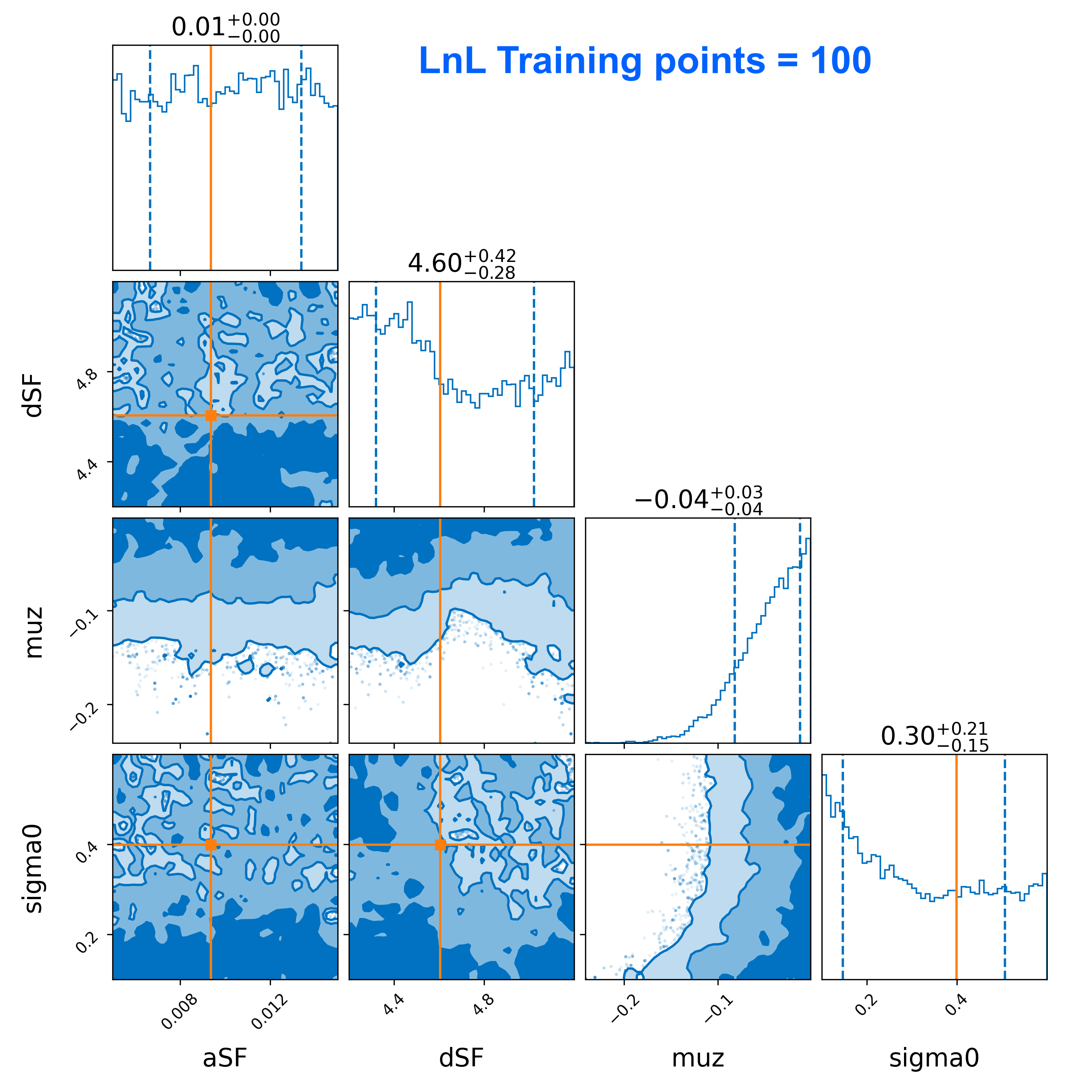
500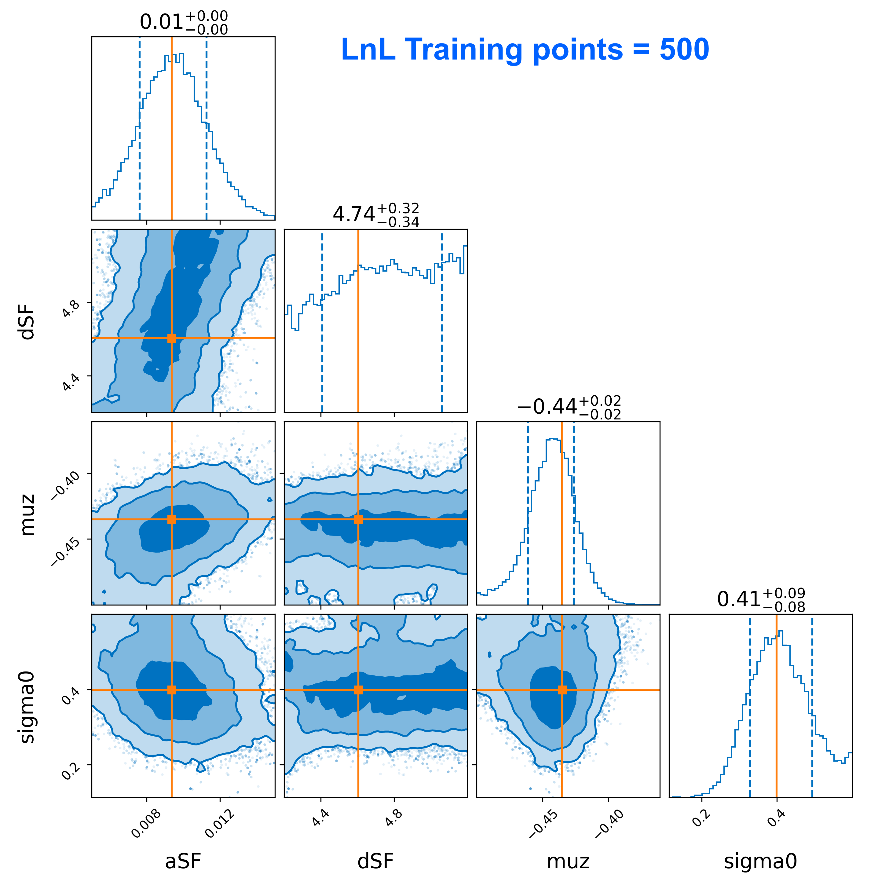
1000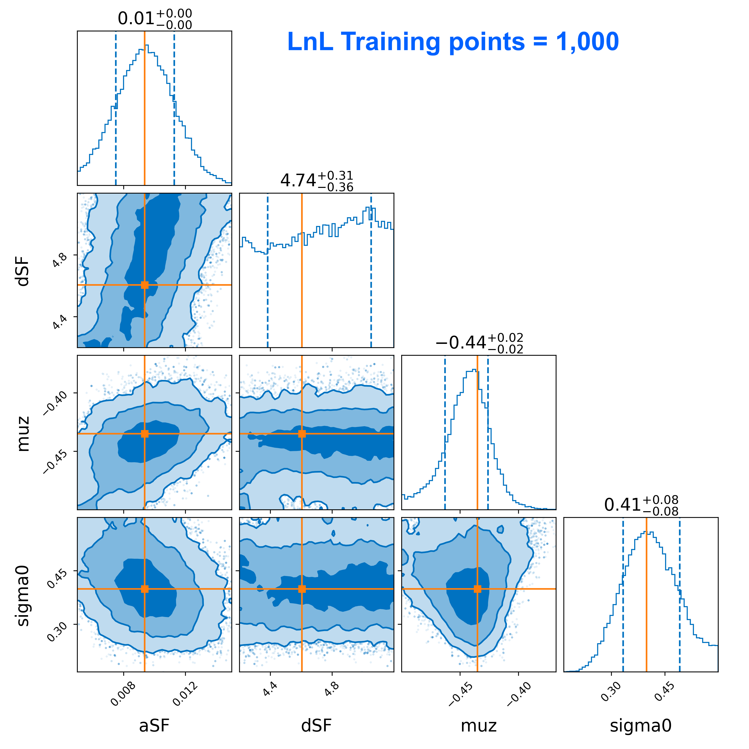

In this case, the surrogate has trained with ~500 training points.

PP Test

Running a PP-test with 100 events (500 training points for each). Still running, but atm

1. Sampler fails for several injection sets
2. Sometimes, the sampler finishes and the posterior looks bogus (maybe we need to increase training data/adaptive sampling).

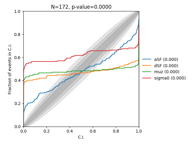This type of pp-plot means we have over-constrained the posterior

Examples:

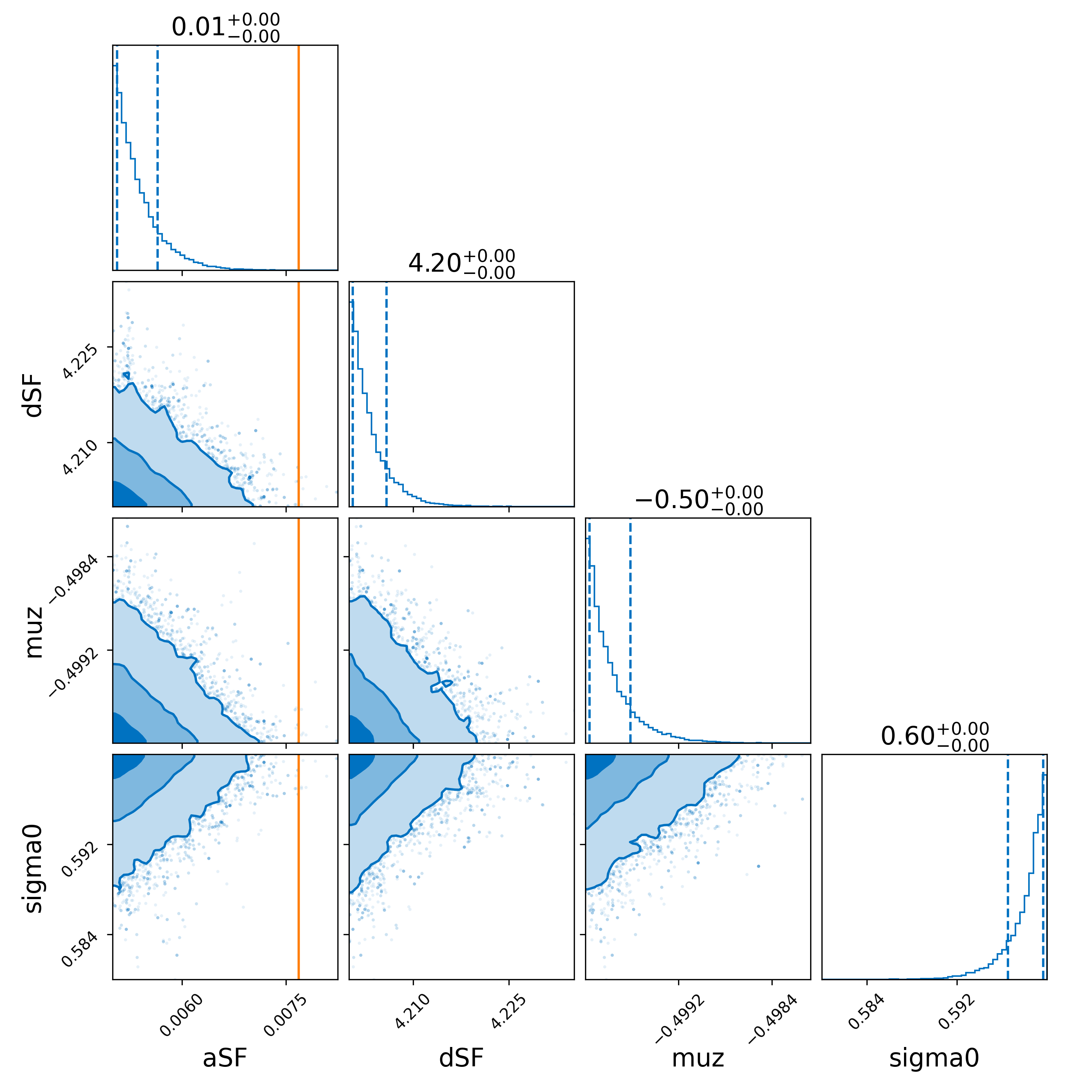
idx	detection-matrix	posterior	comments
628		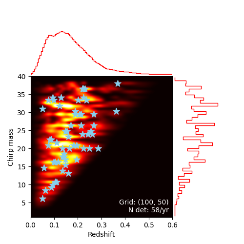	Looks ok..
1071		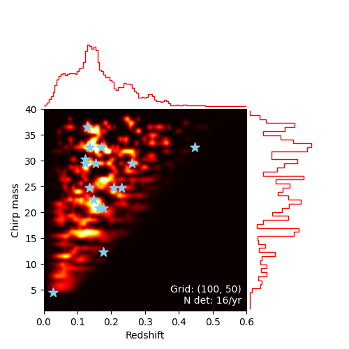	Sampler didn't converge
1892		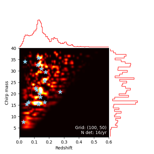	Sampler failed (nburn>nsteps)

Investigating a 'biased' posterior

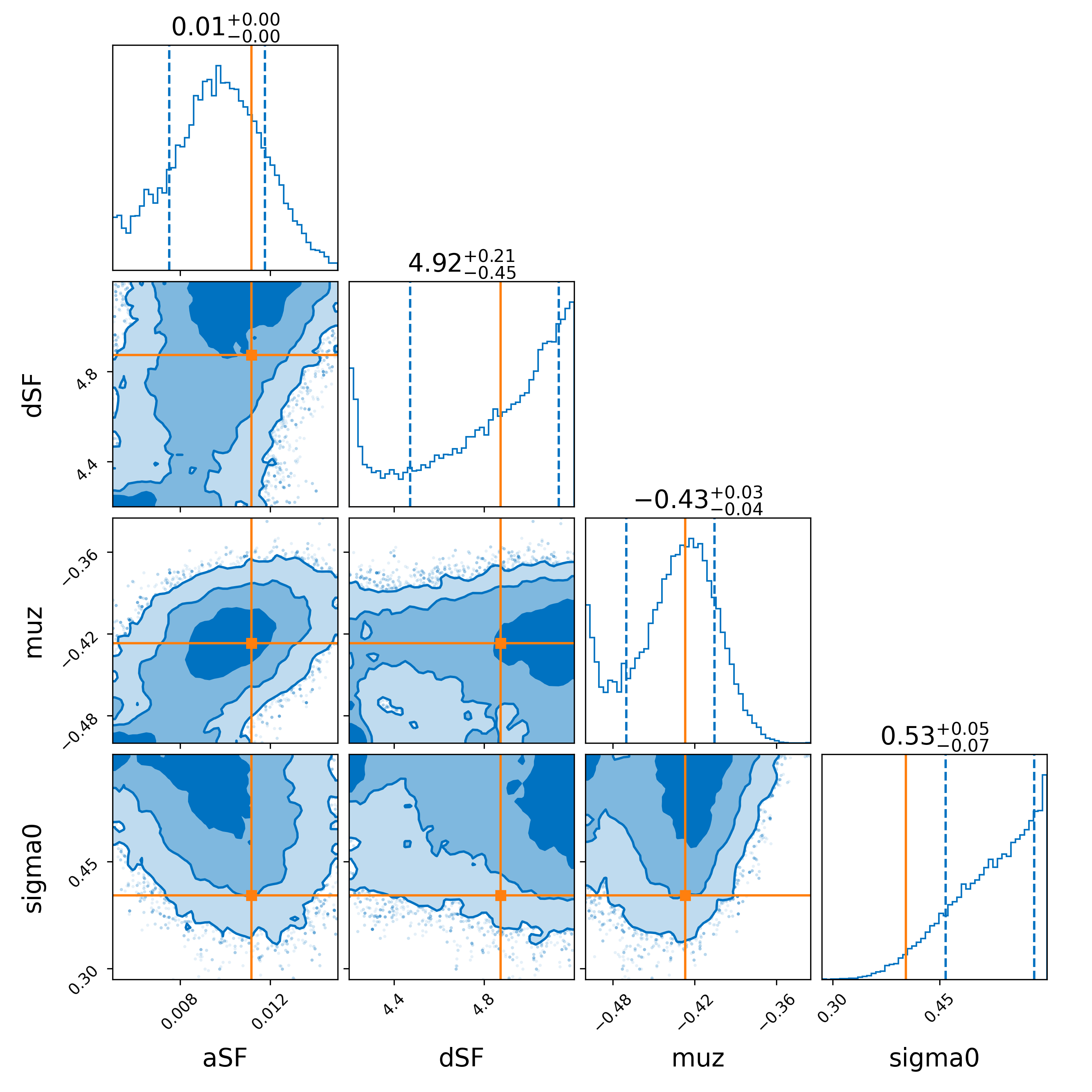
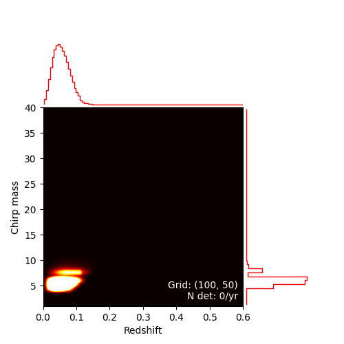
Simulating the following system:

Data	Corner

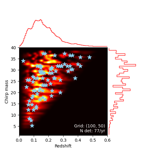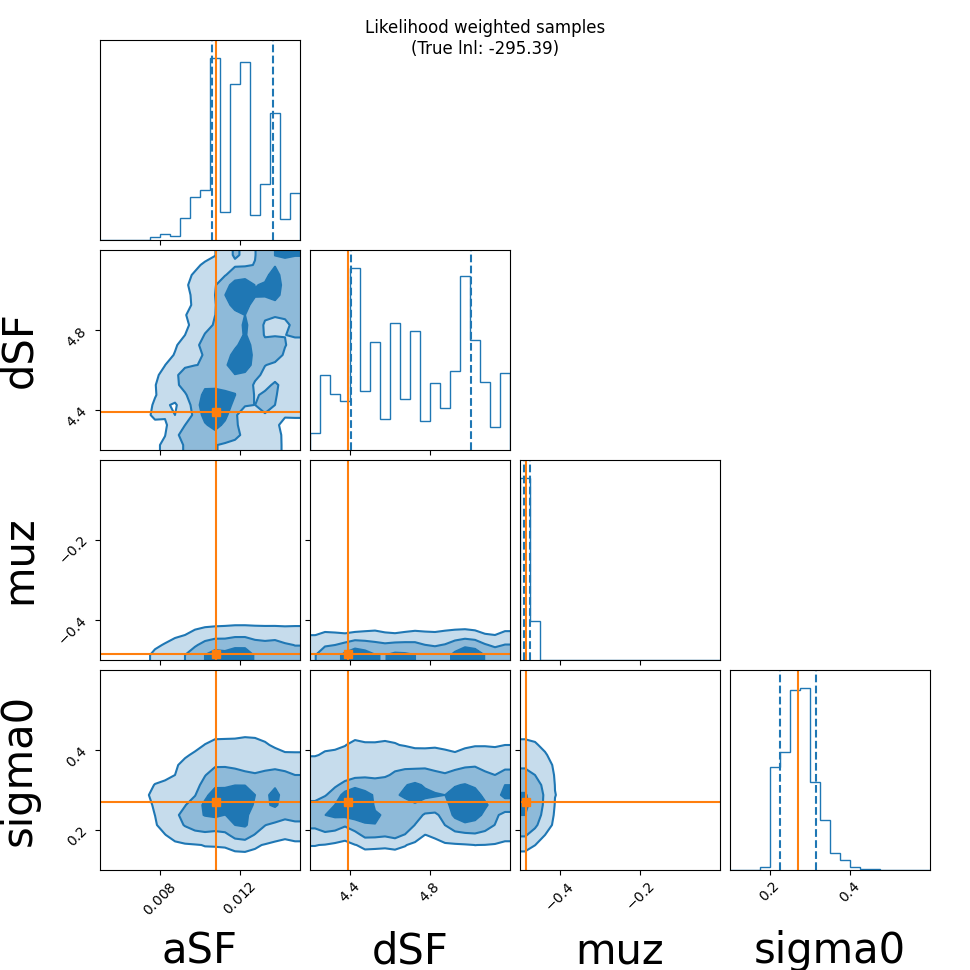THIS IS THE TRUE EVENT -- True Lnl: -295.35

Now, trying to train with different amounts of data:

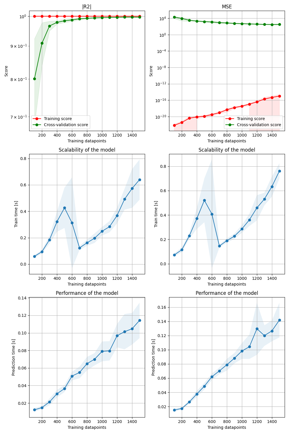
The validation error is really high!!

Here is a plot of the numerical Lnl vs surrogate Lnl when the surrogate is trained with ~400 datapoints:

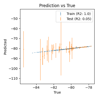
QS FOR ILYA What is the numerical LnL uncertainty? I should try to account for that in the GP (right now I am assuming our numerical LnL measurements are perfect). Unc in COMPAS? Unc in comsic integrator?

Sampling with different trained models (each using more data):

Ntrain	Corner	true - pred LnL
100		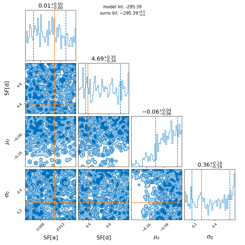0
250		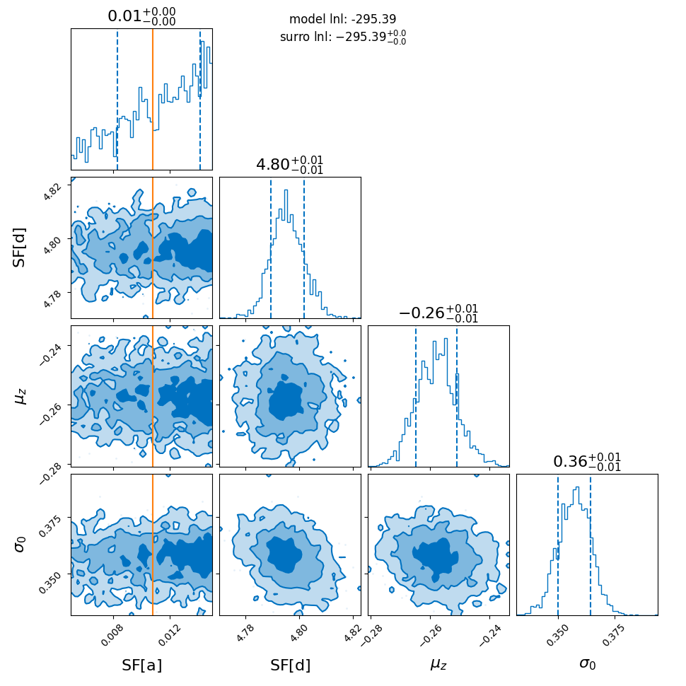0
500		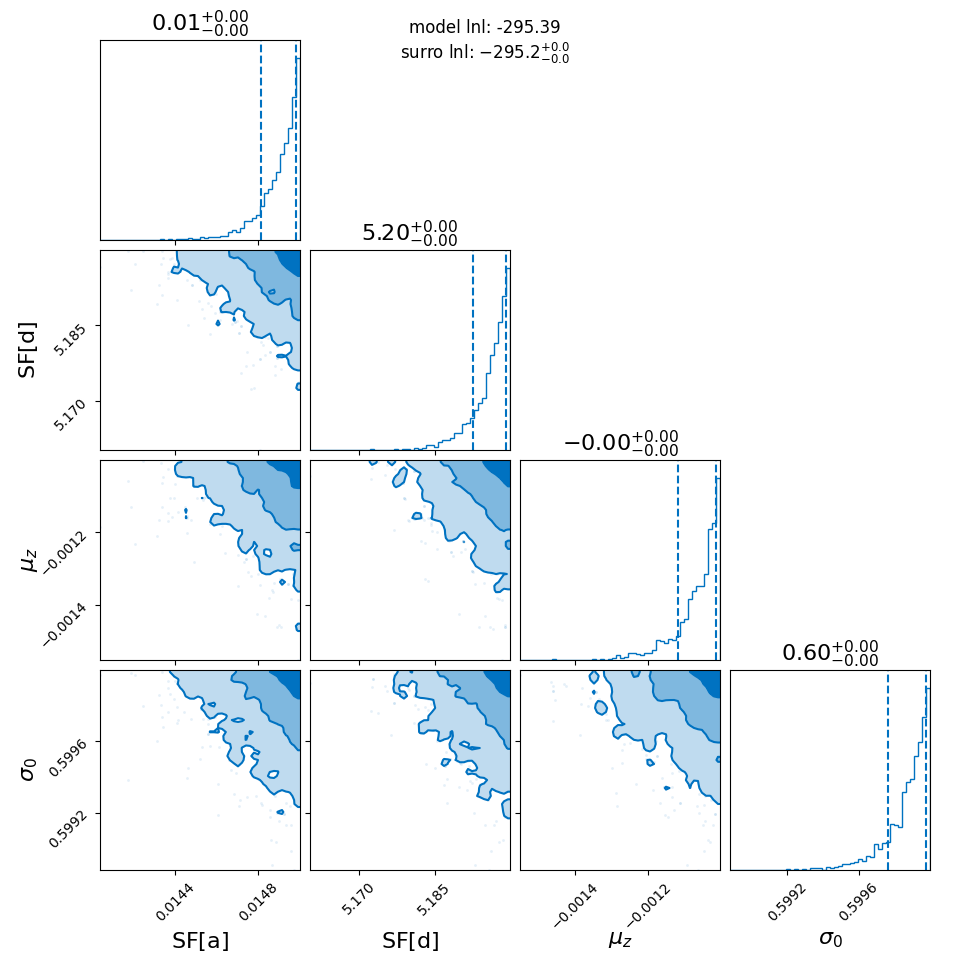0.19
1000		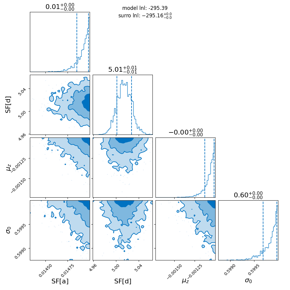0.23

---

inf Lnl bug at high muz values!

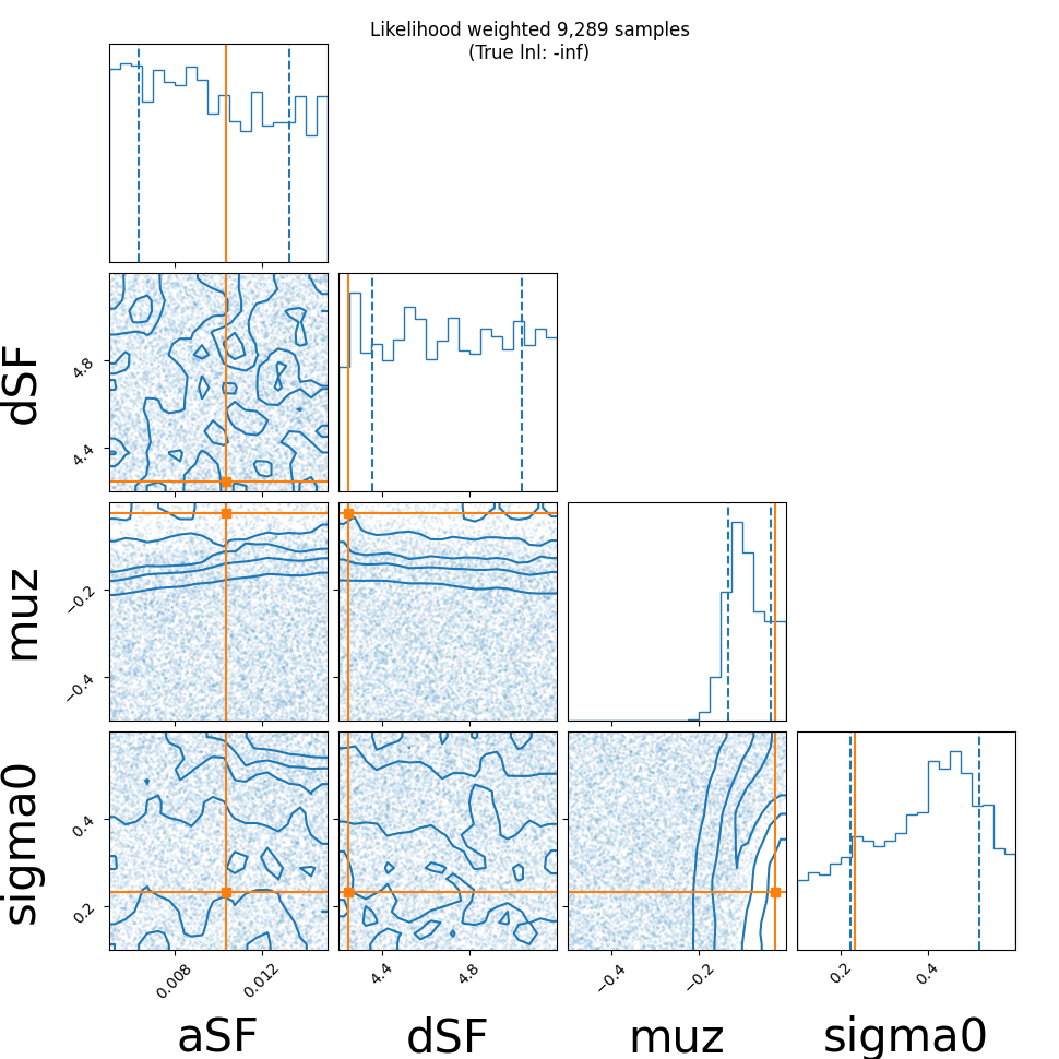
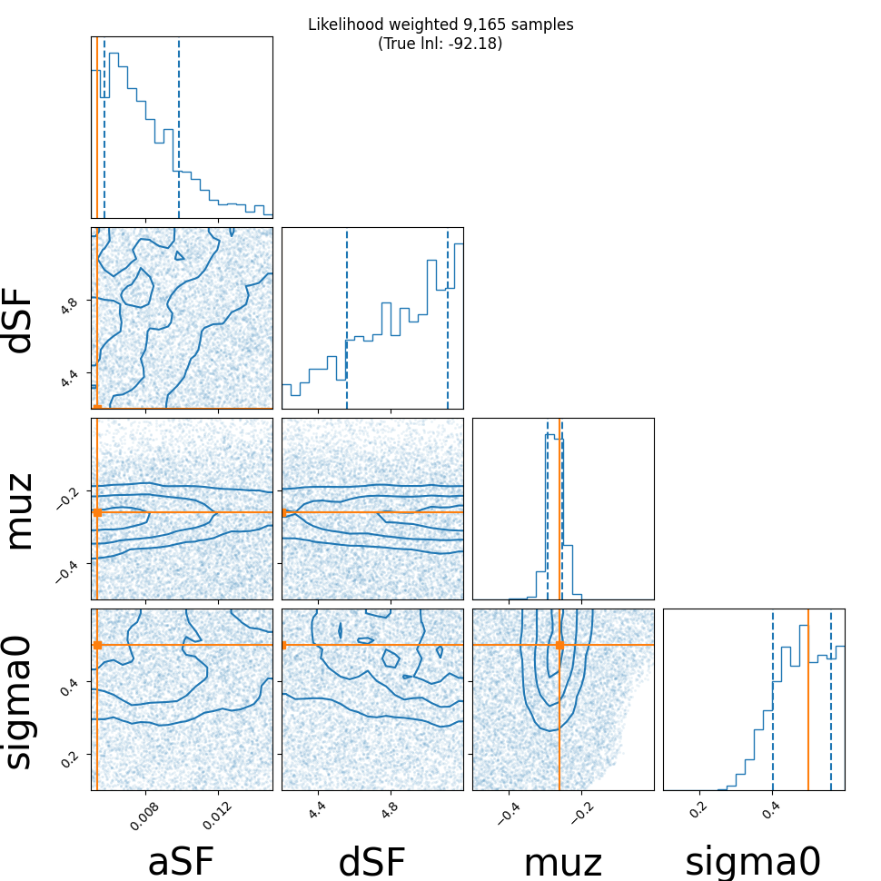
Some regions of the parameter space --> lnl ~ -inf

Uni	Lnl Training Data

---

Investigating model with different numbers of training points

N	pic
100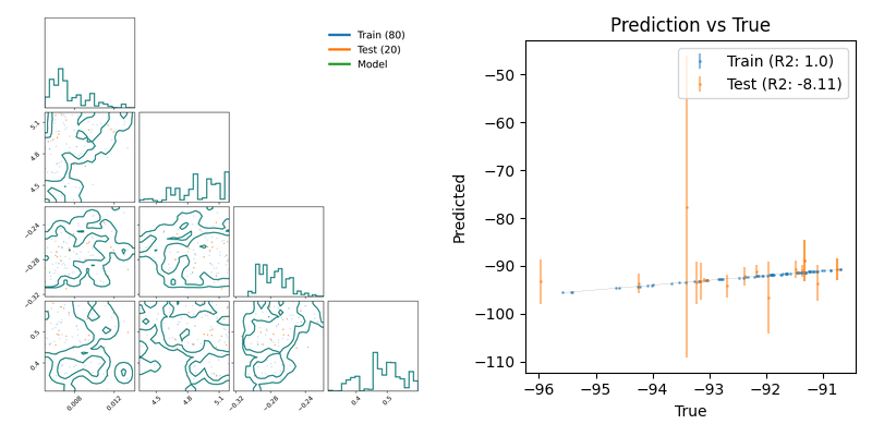
500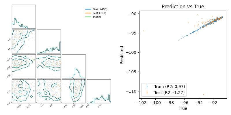
1000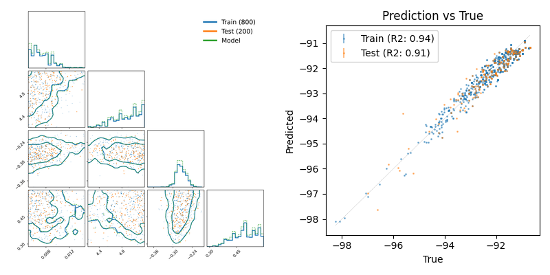
2000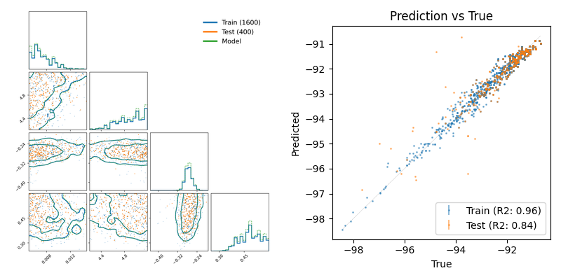