User Guide
Rough guide by Simon Niemeyer
TODO
TODO
Welcome to DeliberateQ. Below I’ve provided a very brief run through of how to do a basic analysis.
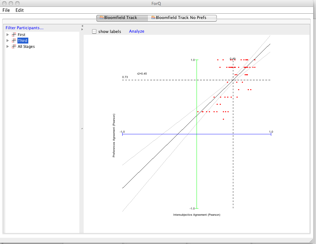
The thing to remember about this software is that it has been developed to do more than what is usually done in Q analysis. For example: I do analyses that combine Q data with preference data to explore the relationships at stages of a longitudinal study (usually before and after deliberation). The figure below shows an example of an Intersubjective Consistency plot. This will not be relevant to most studies.
This version of the program also works Q data along (i.e. without preference data) so it's more accessible for other kinds of users.
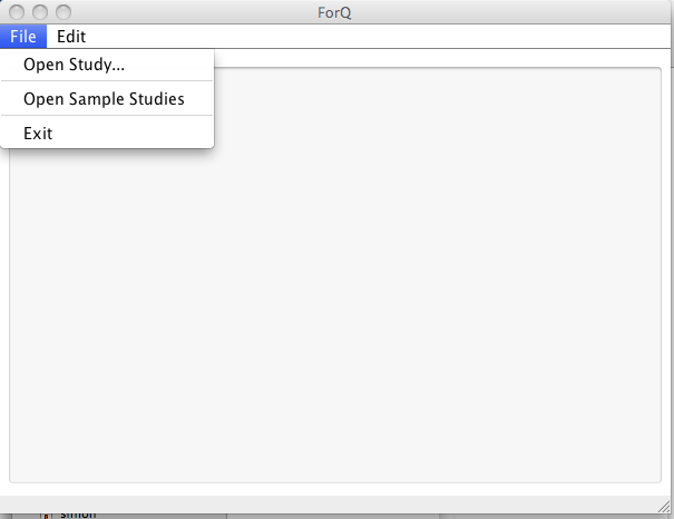
To get familiar with the software, the easiest thing to do is to load the built in data using the file menu (select “Open Sample Studies”) this load the Bloomfield Track case study data.
The file includes data that is broken into two different “stages” of a longitudinal study.
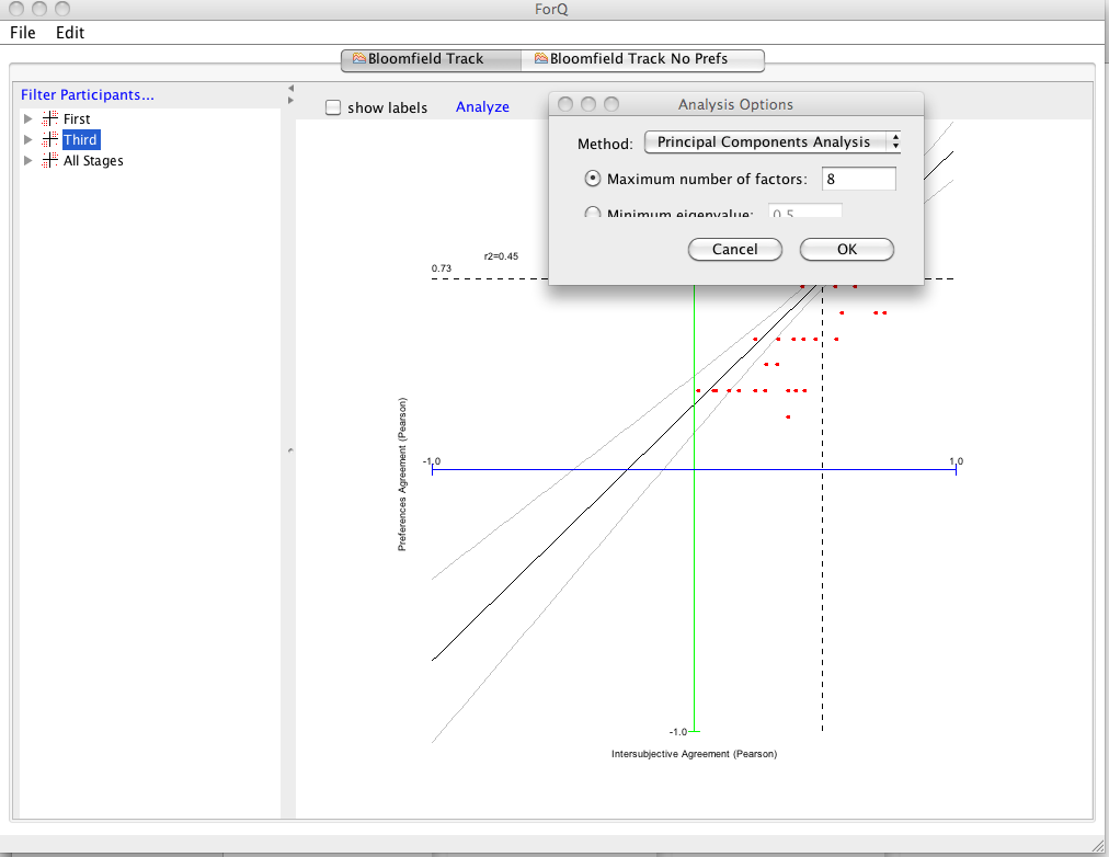
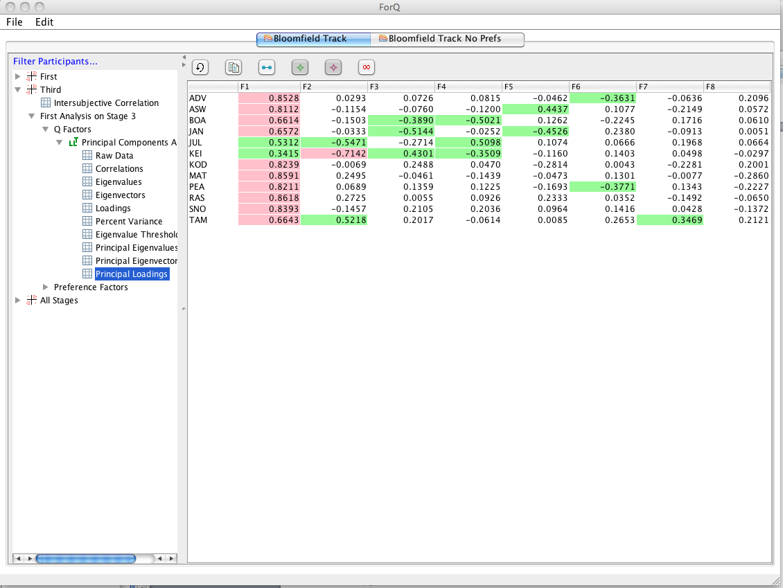
To start the Q analysis you select the data you want to analyze from the LHS window (in this case I’ve selected 'Third' stage data, but in most case you would use “All Stages”). A window with Analysis options pops up and you choose whether you want to restrict the number of factors numerically (in this case 8 factors) or using a minimum Eigenvalue.
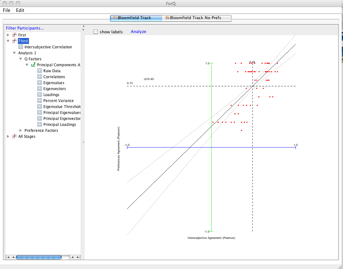
The analysis will then appear in the LHS window (you'll need to click the arrows to expand the details). Note that you can do multiple analyses and assign names to each by double clicking the heading. Subsequent analyses will appear in order in the LHS window.
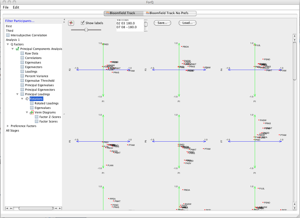
If you want to go and and perform further rotations, select the “Principal Loadings” in the LHS window that you want to rotate and click the Rotation button (indicated by the arrow below).
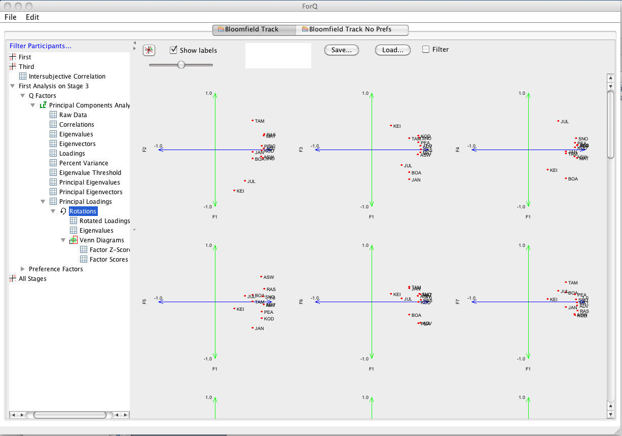
Now you’ll see the RHS window change to show all combinations of factor loading plots. This is the window that you use to do the rotations. (Note that you can navigate to and from it in the LHS window). If there are a lot of factors you will need to scroll around the window to see them all. You can also scale the graphs using the slider in the RHS window. You can also select to show labels (you can also filter out certain data points, depending on how the data input file is set up…but I won’t go into that for now.) Now you can use this window to do standard mathematical rotations and/or theoretical rotations. You can choose the type of mathematical rotation you want to do using the button in the top LH of the RHS window
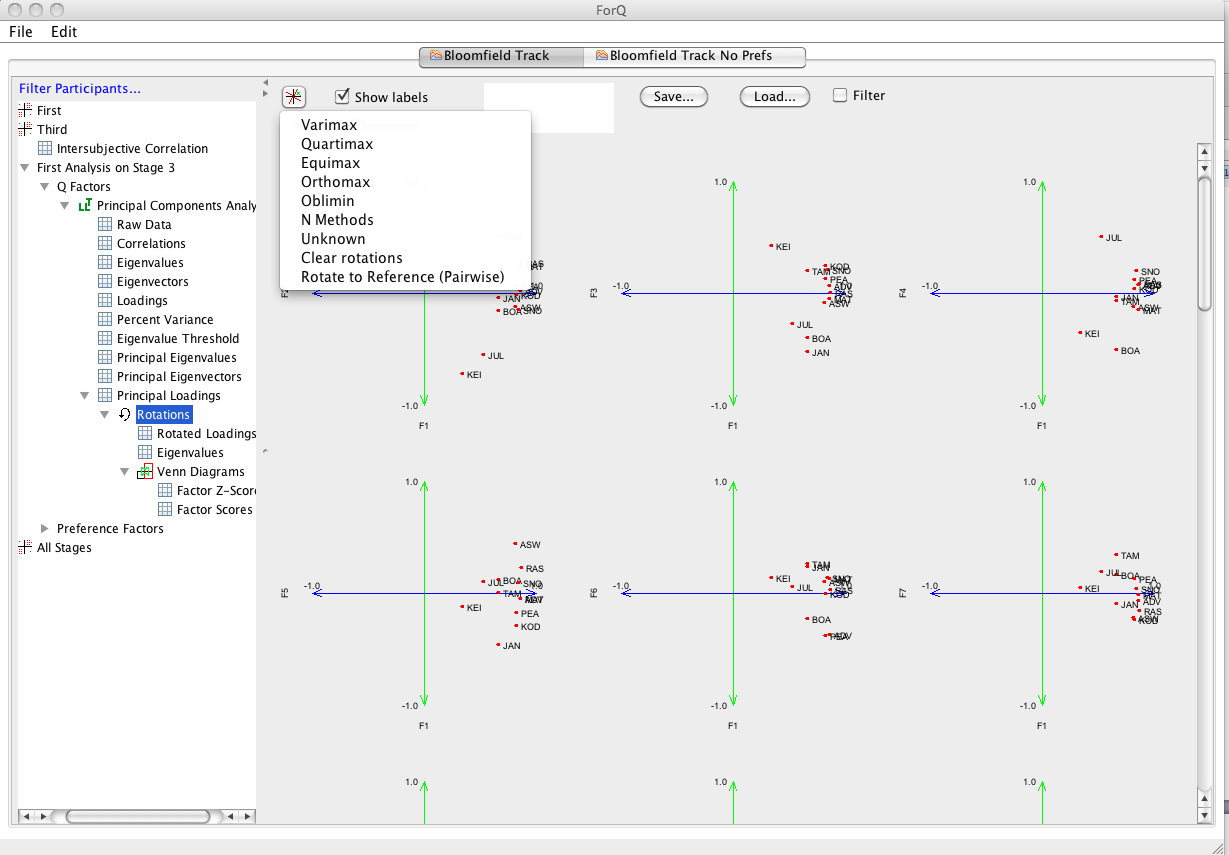
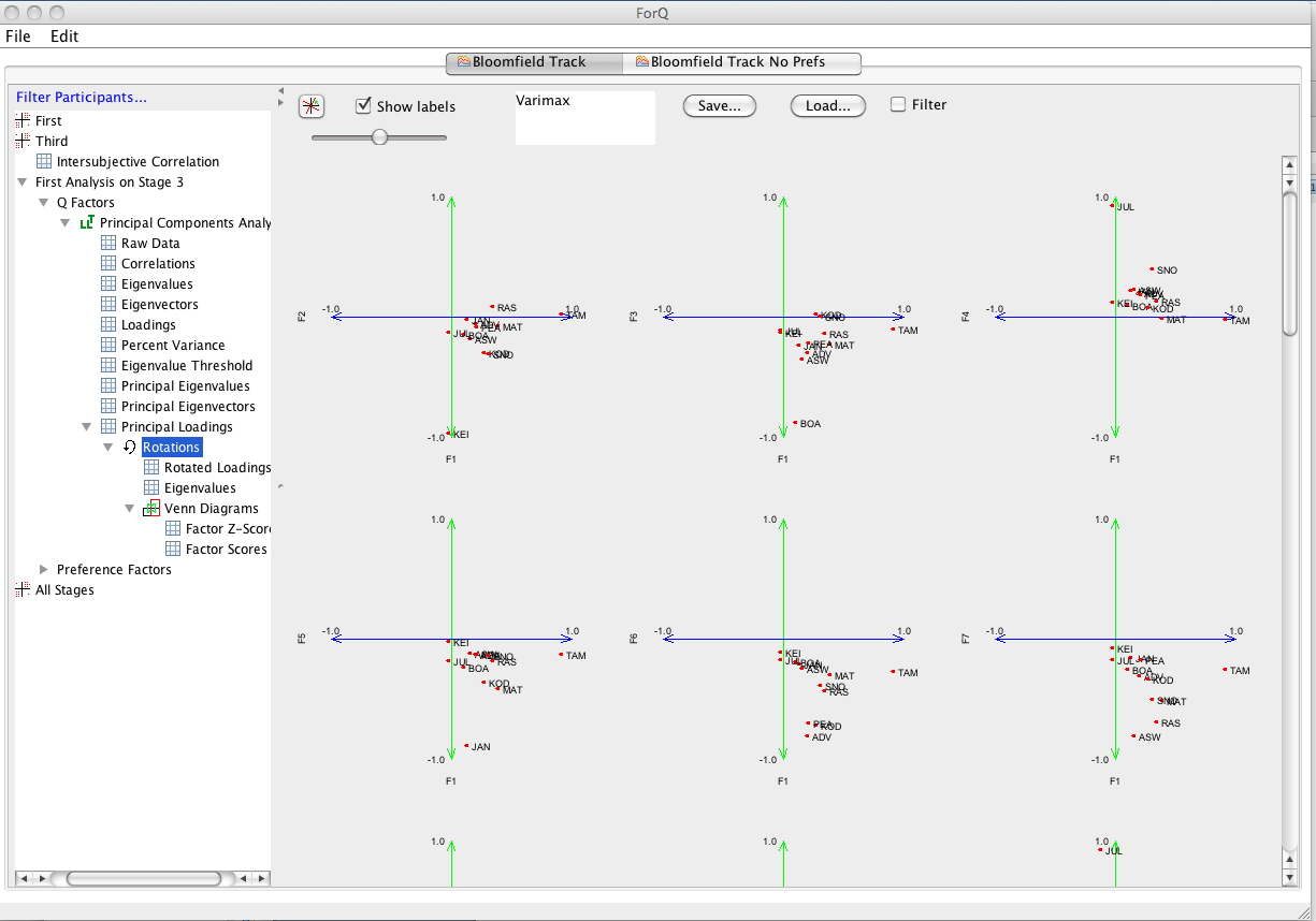
You’ll see below that there are many methods that can be used to rotate (Varimax being by far the most common). There are a few options that are developmental (unknown and Rotate to Reference). The other main option you need to note is Clear Rotations, which takes you back to the start of the rotation process.
You’ll see in the RHS window that there will appear a list of rotations that you’ve performed so far, which you can also use to track the angle of the rotation that you’re currently performing.
Now, at any stage you can go in and have a look at the impact that the rotations are having on the factors. You can do this by using the LHS window to the different types of output that Q method produces (Factor Loadings, Factor Scores). You can also use the Venn Diagram option to have a quick look at how the statements distribute across factors. An example is shown below. Note that this window is also used to set the way in which sorts are selected to perform factor scores. At this stage we don’t have a facility for manually selecting sorts associated with each factor (we’re working on it). Instead you can choose a strategy for selecting sorts. You need to begin by choosing the strategy from the drop down list. The default strategy is simply to choose any Q sort that has a unique significant loading on a factor (exclude confounding sorts). You can also relax the strategy to sorts that might have a significant loading on one other factor (Ignore all participants with more than two significant factor loadings); or you can use all Q sorts with a significant loading. The other important option here is the level of significance that you use to select sorts. You can adjust this using the “Confidence” and ‘Threshold” sliders at the top of the window. You can use Confidence slider to set the significance level and then the LH Threshold slider to multiply the resulting threshold. E.g. when the left slider is set at 95% and the RH slider at 1.00, the threshold is 0.28. (Now this is a bit cumbersome and we need to work on it. And currently you can’t see the Confidence level because the font is too big: which is set at a default of 95%) The easiest thing to do is just use the RH threshold slider and use the threshold level for the factor loading (here 0.28).
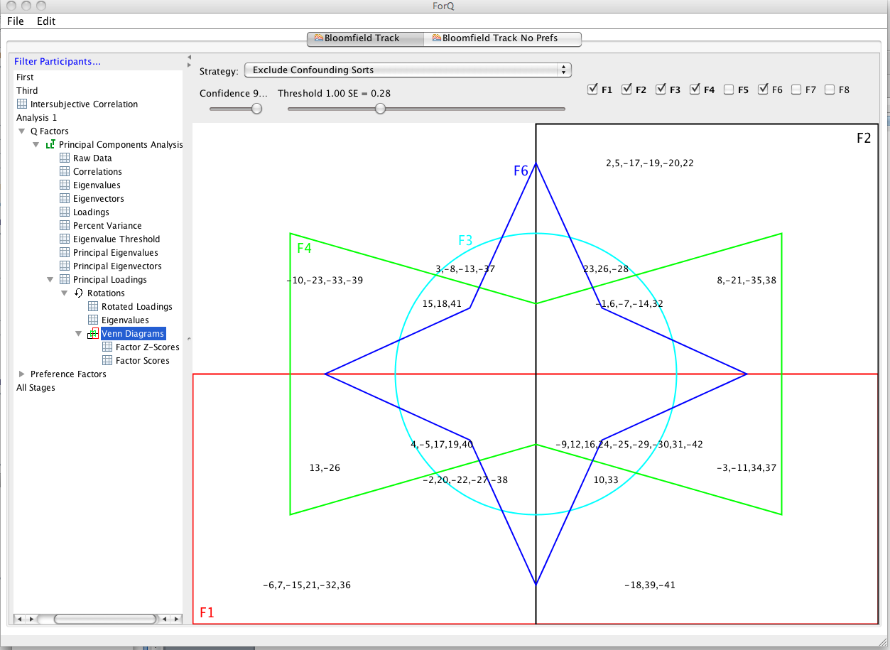
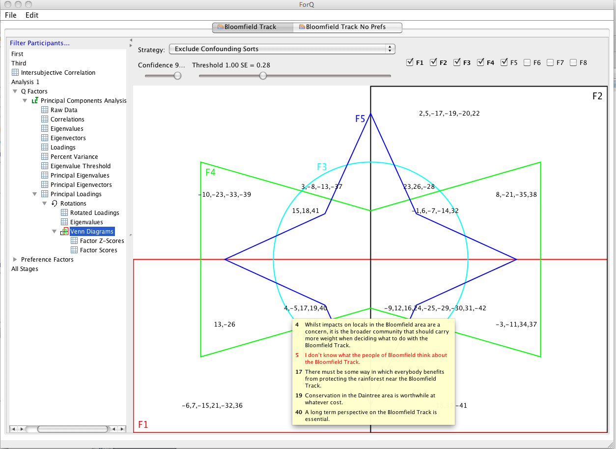
Using the Excluding Confounding Sets at a threshold of 0.28 produces five viable factors that have non-confounding Q sorts with a loading over 0.28 (1, 2,3,4 and 5). In the Venn diagram window these viable factors are shown in bold in the top right of the RHS window. The Venn diagram can only show five factors at a time. You need to select which five you want to look at be checking the box next to the factor number in the top right of the RHS window. In the figure 1,2,3,4 and 6 are selected, but factor 6 is an empty set, because it doesn’t have any viable Q sorts under the no-confounding-sort/0.28 threshold strategy. For those factors that are viable, you can have a quick look at the statements associated with each factor by holding the cursor over the list of statements, which will produce a pop up window with the complete statements (see figure below).
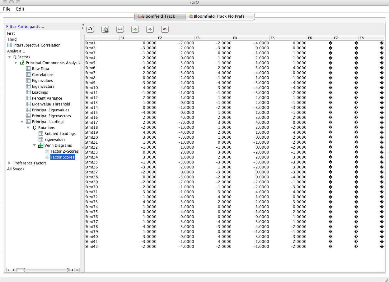
You can also go and look directly at the factor scores (or Z scores) for each factor that are produce using the strategy you’ve chosen in the Venn diagram window. The figure below shows the Factor Score window for this analysis. You’ll see a list of scores for each statements (rows) for each of the factors (columns). (We need to fix the zeros.) If you want to copy this data to put into another document (e.g. Excel), just click the copy button at the top of the RHS window (indicated by the arrow). You can do the same for any window that contains data. For now, this is how you obtain the results of the analysis, because the program does not produce reports at this stage (and will be unlikely to in this round of development). Note that only the first five factors produce factor scores, because the other factors do not have any viable Q sorts using the strategy chosen in the Venn Diagram window.
OK, that’s the main points covered. You can keep going from here, adding extra analyses simply by going back and selecting the data you want to use at the top of the LHS window. You can also add different rotation strategies to the same analysis by (re) selecting the Principle Loadings window from the LHS Window and (re)clicking the rotation button. Additional analysis/rotations just get added to the list in the LHS window. There are a number of features that I haven’t mentioned, which shouldn’t be required from most. But you can get a sense of what can be done by having a play around with the program.
TODO
By default DeliberateQ uses Spearman's correlation coefficient. To specify another type, add a system property on startup:
java deliberate-q.jar -Dcc=PEARSONSValid values for the cc option are PEARSONS, SPEARMANS, CONCORDANCE.