Vehicle Routing Problem (VRP)

Info about the project

Team formed by :

• Iacob Marcel-Emanuel (2B4) - responsible for implementing the algorithm for solving the VRP
• Logofatu Ionut-Nicusor (2B4) - responsible for developing the desktop interface

Project for Advanced Programming Laboratory (2020 - 2021), Faculty of Computer Science Iasi
Lab coordinator: Irimia Cosmin.

Introduction:

The Vehicle Routing Problem is a combinatorial optimization problem which appeared in 1959, in an article written by George Dantzig and John Ramser, which poses the question: "What is the optimal set of routes for a fleet of vehicles to traverse in order to deliver to a given set of customers?".
It generalises the well-known travelling salesman problem (TSP), which is a well known problem in the NP-Hard class (so determining the optimal solution to VRP is NP-hard). Therefore, commercial solvers tend to use heuristics due to the size and frequency of real world VRPs they need to solve.

Formal definition:

We are given a number n of vehicles, each one of them having a limited capacity (measurable by weight in our case), and m destinations, each one of them having zero, one or more packages with varying weights. Having the coordinates for each destination (in euclidean 2D distance), we wish to determine the path each vehicle should take in order to deliver all the packages and have the minimal cost for the company.

Simulated Annealing (SA) Algorithm (used for TSP)

Firstly, we should talk about Simulated Annealing. Simulated annealing can be used for very hard computational optimization problems where exact algorithms fail; even though it usually achieves an approximate solution to the global minimum, it could be enough for many practical problems.

The basic idea is that we initialize the temperature with a high value, which we gradually reduce overtime. At a high temperature, the probability of allowing an upward move is very high, whereas at a lower temperature we have a smaller chance of this happening.

The idea behind annealing is that at high temperatures, our candidate solution should jump out of a local minimum, allowing us to continue our search on a wider array of values. The algorithm uses an initial temperature that gradually cools over time, restricting the algorithm to choose a worse neighbor that could lead to a better solution over time. The candidate solution is represented by a permutation of the destinations, as we can get to any destination from any other destination. Using the greedy hybrid operator proposed by Wang, we can obtain decent results (values very close to the optimum on small instances). We use this operator to produce a new candidate solution.

The neighbor of a candidate solution is defined as the minimum of the inverse, insert and swap operators.

• Inverse: This operator reverses the order of the numbers (destinations) in our original permutation between two random positions, i and j.
• Insert : This operator moves the destination in the randomly chosen position j to the randomly chosen position i.
• Swap : This operator swaps the destination from the randomly chosen position i with the destination on the randomly chosen position j

These operators are applied to every candidate solution that we get. The cost of the edges between the nodes chosen is calculated, then the smallest of the three is compared with the current solution.

Setup

• Initial temperature T: 100
• Number of iterations t: 1000
• Termination condition: 10 ^ (-8)
• Temperature modification: T = T * 0.99

Proposed solution:

Using the aforementioned algorithm, we can implement it in our VRP algorithm so it can help us solve it. Here are the steps simply explained:

• We start with the first car.
• Using TSP, we determine the shortest path it can take from the depot (this is destination 1 at all times) to all other destinations (and its cost).
• We fit in as many packages as possible for the destinations in the car's path.
• We remove the destinations which have all the packages delivered.
• The cost of this trip will be equal to the cost of visiting all the possible destination times two (counting returning to the depot to get other packages).
• We proceed with the next car.
• Using TSP, we determine the shortest path it can take from the depot to all other unfinished destinations.
• We cycle through all cars until all the packages are delivered.

This solution guarantees that the cars will take the shortest path possible (determined by SA) at any time.

JavaFX

For desktop interface we used JavaFx because we can manipulate data easily.

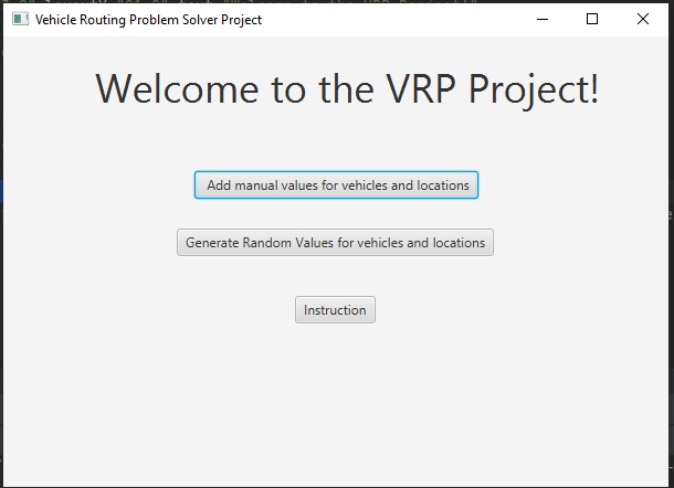
When you run the program will appear one scene with three buttons

• Add manual values for vehicles and locations

• Generate Random Values for vehicles and locations

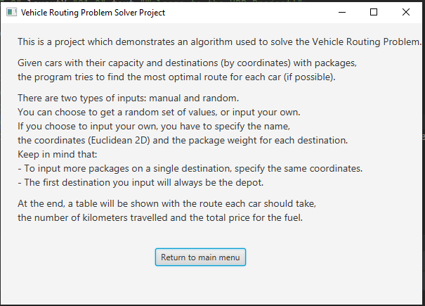
• Instruction

• When you click on the instruction button, you will see what rules this application has. The instruction scene will look like this.

  

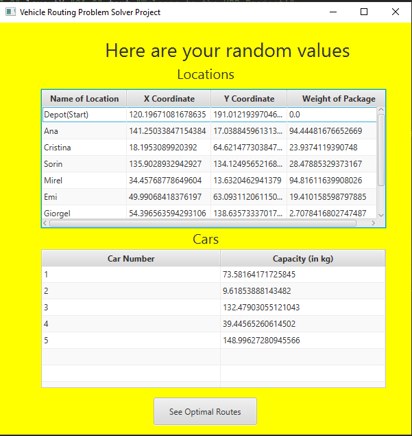
• On the Generate Random Values scene you will see some random values generated by our program for locations and cars. After we generate and display them, we will write them in different files and will call the function that will determine the solution. After we have the solution, we will write it in one file because we need to display it on the next scene.

  

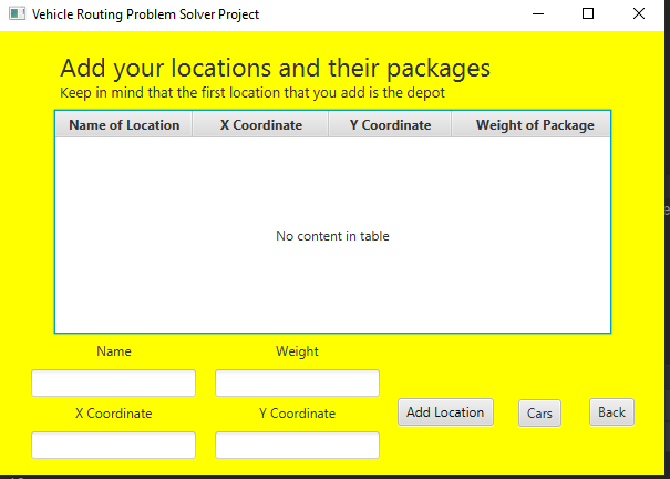
• When you click on the Add manual values, the next scene will appear and you can add how many location do you want. Keep in mind that the first location will be the depot, so should not have the weight value.

  

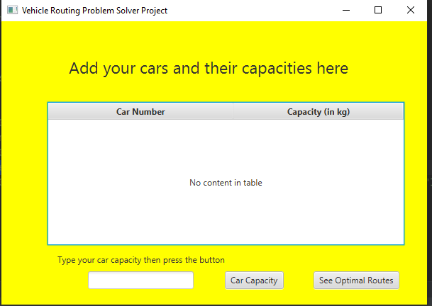
• After you added manual values for location, next you need to add manual values for cars weight.

  

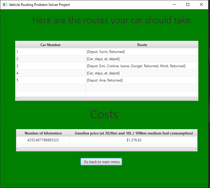
• When you click on the results, the program will write all your data in different files and will call the function that will determine the solution. After we have the solution, we will write it in one file because we need to display it on the next scene.

  

• As you can see, here is the solution and the total amount that should be spent depending on how many kilometers the cars have traveled.