In this exercise, you will implement the backpropagation algorithm to learn the parameters for the neural network.

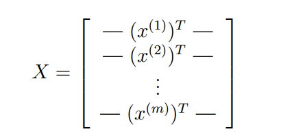
This is the same dataset that you used in the previous exercise. There are 5000 training examples in ex3data1.mat, where each training example is a 20 pixel by 20 pixel grayscale image of the digit. Each pixel is represented by a floating point number indicating the grayscale intensity at that location. The 20 by 20 grid of pixels is \unrolled" into a 400-dimensional vector. Each of these training examples becomes a single row in our data matrix X. This gives us a 5000 by 400 matrix X where every row is a training example for a handwritten digit image
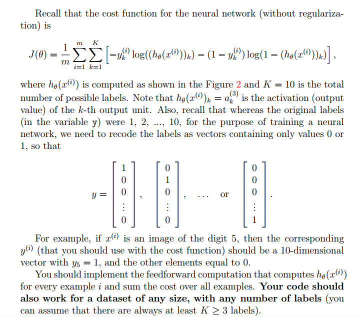
The second part of the training set is a 5000-dimensional vector y that contains labels for the training set. Therefore, a \0" digit is labeled as \10", while the digits \1" to \9" are labeled as \1" to \9" in their natural order
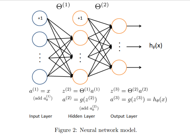
Our neural network is shown in Figure 2. It has 3 layers { an input layer, a hidden layer and an output layer. Recall that our inputs are pixel values of digit images. Since the images are of size 20 × 20, this gives us 400 input layer units (not counting the extra bias unit which always outputs +1). The training data will be loaded into the variables X and y by the ex4.m script. You have been provided with a set of network parameters (Θ(1); Θ(2)) already trained by us. These are stored in ex4weights.mat and will be loaded by ex4.m into Theta1 and Theta2. The parameters have dimensions that are sized for a neural network with 25 units in the second layer and 10 output units (corresponding to the 10 digit classes).
Implementation Note: The matrix X contains the examples in rows (i.e., X(i,:)’ is the i-th training example x(i), expressed as a n × 1 vector.) When you complete the code in nnCostFunction.m, you will need to add the column of 1’s to the X matrix. The parameters for each unit in the neural network is represented in Theta1 and Theta2 as one row. Specifically, the first row of Theta1 corresponds to the first hidden unit in the second layer. You can use a for-loop over the examples to compute the cost. Once you are done, call your nnCostFunction() using the loaded set of parameters for Theta1 and Theta2. You should see that the cost is about 0.287629.
In this part of the exercise, you will implement the backpropagation algorithm to compute the gradient for the neural network cost function. You will need to complete the nnCostFunction.m so that it returns an appropriate value for grad. Once you have computed the gradient, you will be able to train the neural network by minimizing the cost function J(Θ) using an advanced optimizer such as minimize. You will first implement the backpropagation algorithm to compute the gradients for the parameters for the (unregularized) neural network.
When training neural networks, it is important to randomly initialize the parameters for symmetry breaking. One effective strategy for random initialization is to randomly select values for Θ(l) uniformly in the range [−EPS_init; EPS_init]. You should use Eps_init = 0:12.2 This range of values ensures that the parameters are kept small and makes the learning more efficient. RandInitializeWeights() is initialize the weights for Θ;

After the training completes, script will proceed to report the training accuracy of your classifier by computing the percentage of examples it got correct. If your implementation is correct, you should see a reported training accuracy of about 95.3% (this may vary by about 1% due to the random initialization). It is possible to get higher training accuracies by training the neural network for more iterations. We encourage you to try training the neural network for more iterations (e.g., set MaxIter to 400) and also vary the regularization parameter λ. With the right learning settings, it is possible to get the neural network to perfectly fit the training set.