This is my Python implementation of the A* pathfinding algorithm. The application is written in Python using Kivy as well as PIL (Python Imaging Library) for the GUI.
Download the latest release and follow the install instructions or download the source code and run Main.py from an IDE
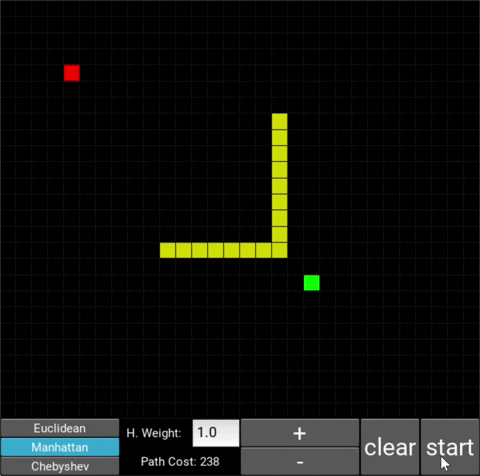
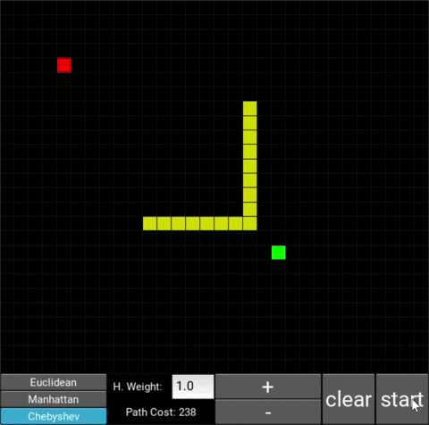
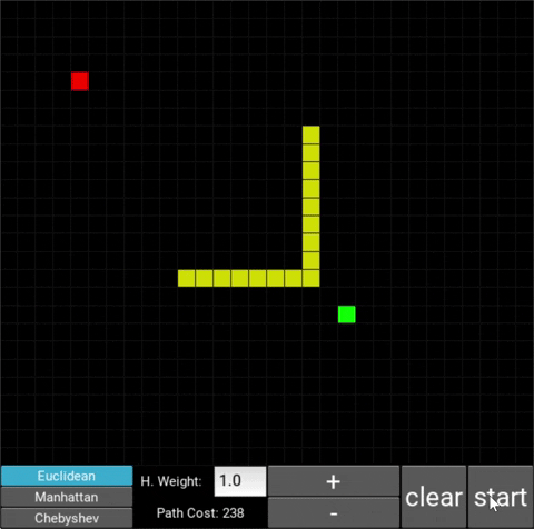
- The red/green squares represent the starting/goal node respectively.
- You can move the starting/goal node by clicking on it and then clicking on some desired square (where you want to move the node to).
- You can use the mouse cursor to draw obstacles onto the grid (in yellow).
- You can erase a drawn obstacle square by clicking on it again.
- To start the algorithm, click on the "Start" button.
- Clicking on "Clear" once erases the path drawn by the algorithm.
- Clicking on "Clear" a second time also erases the obstacles.
- Zoom in/out by clicking on the +/- buttons.
- You can select one of the distance metrics by clicking on the respective button (Euclidean, Manhattan, Chebyshev)
- You can enter a new heuristic weight into the input box
- After the path has been traced, the total cost is being shown in the "Path Cost" box
Each cell on the grid, also called a "node" can be:
- "Explored", node that the algorithm already visited (neon pink cells)
- "Unavailable", node that the algorithm has not seen yet (black cells)
- "Available", node that the algorithm is aware of but hasn't visited/explored yet (dark pink cells)
There are also obstacle cells (yellow cells) which the algorithm cannot visit. Upon finding the goal node, the path is traced back to the starting node.
When a node becomes "available", it is assigned 3 values:
- F Cost, G Cost and H Cost , where F Cost = G Cost + H Cost,
- G Cost is the cost from that node to the starting node.
- H Cost is the approximated cost from that node to the goal node. (also called the heuristic function)
This heuristic function will allow A* to give preference to nodes that are closer to the goal node, which saves a lot of time.
Each frame, the algorithm will look at all the "available" nodes and visit/explore the one with the lowest F Cost. This will then repeat until the algorithm has arrived at the goal node. Generally, by always picking the lowest F Cost, the overall cost of the path will be kept as low as possible, which will find you the shortest path (although only under certain conditions, as we'll see).
One unique feature of my implementation is that the H Cost is always being multiplied by some weight (heuristic weight), which the user can change. This weight enables the user to change the behaviour of the search algorithm, so actually:
F Cost = G Cost + H Cost * Weight
(for more details see: https://en.wikipedia.org/wiki/A*_search_algorithm, https://en.wikipedia.org/wiki/Dijkstra%27s_algorithm).
- This is the standard configuration, which is the classic A* search algorithm. The heuristic weight is set to 1. With this heuristic, the shortest path will always be found. You can also choose from 3 distance metrics, which are used to calculate the distance between two nodes: Euclidean, Manhattan and Chebyshev.
(Note: these GIFS are not representative of the real framerate/resolution of the application, due to image compression)
Euclidean:

Manhattan:

Chebyshev:

- By setting the heuristic weight to 0, you remove the heuristic function. This reverts the A* algorithm back to Dijkstra's algorithm which essentially is still A*, just without the H Cost/heuristic. Dijkstra's algorithm will always find the shortest path, although it will take substantially longer than A*:
- By changing the heuristic weight, the algorithm behaves differently. But why?
As described above, F Cost = G Cost + H Cost * Weight
Each frame, the algorithm will explore the node with the lowest F Cost.
If we set the heuristic weight > 1, the H Cost * Weight term will start to "outweigh" the G Cost. This means that each frame, the node with the lowest F Cost will likely just be the one with the lowest H Cost (closest to the goal node). The more we increase the heuristic weight, the more G Cost becomes negligeable. What does this mean in practice?
Effectively, the algorithm will spend less time exploring other directions (that don't go into the direction of the goal node) which will often result in a shorter runtime, however it may not find the shortest path that exists anymore. This behaviour will become increasingly apparent as the heuristic weight gets bigger.
If we set the heuristic weight < 1, the G Cost will start to "outweigh" the H Cost * Weight term. Each frame. the node with the lowest F Cost will likely just be the one with the lowest G Cost (closest to the starting node). As expected, the more we decrease the heuristic weight, the more H Cost becomes negligeable. In practice, the algorithm will prioritize nodes that are closer to the starting node, making it explore nodes more "radially" into every direction. This has the advantage that the algorithm is more likely to find the shortest path, however the runtime is often longer.
With a heuristic weight = 1, neither the G Cost, nor the H Cost are more important than the other. In fact, they are inversely proportional and balance each other out as when the algorithm comes closer to the goal node, the H Cost decreases while the G Cost increases by the same factor. This is the standard A* algorithm.
The changes in behaviour are gradual. Below is the evolution of the algorithm with heuristic weights 0, 0.2, 0.8, 1, 1.2, 1.5 and 10 .


One can see that when the weight is 10, the path is clearly not the shortest one that exists. This is confirmed by looking at the path cost. For weights 0, 0.2, 0.8, 1, 1.2 and 1.5 the cost is 238, however for weight 10, the cost is 262. While the path is more expensive, it is found quicker than the others.
We can draw a general conclusion from this:
- A smaller heuristic weight results in a longer runtime but cheaper path
- A bigger heuristic weight results in a smaller runtime but more expensive path
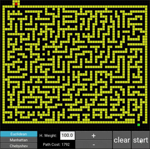
However, this is more of a general guideline and does not strictly apply to every case, as there are limits to it. This can be seen in the practical example below.
This is a labyrinth that I drew.
The respective costs are 944 (weight: 1.0), 1102 (weight: 10.0) and 1729 (weight: 100.0). One notices that with a weight of 10, the algorithm works significantly faster but the path is slightly more expensive (as expected), however if we increase the weight excessively (weight of 100), the runtime gets longer again and the path much more expensive. This shows that a heuristic weight that is too large can slow the algorithm down again.
In this case, the optimal weight would be 10 as it balances speed and cost the best:


-
Python 3.x
-
Kivy 2.0.0
-
PIL (Python Imaging Library)
- https://en.wikipedia.org/wiki/A*_search_algorithm
- https://en.wikipedia.org/wiki/Dijkstra%27s_algorithm
- https://www.youtube.com/watch?v=-L-WgKMFuhE
- http://theory.stanford.edu/~amitp/GameProgramming/Heuristics.html
- https://qiao.github.io/PathFinding.js/visual/
- https://www.redblobgames.com/pathfinding/a-star/introduction.html
- https://wikimedia.org/api/rest_v1/media/math/render/svg/2e0c9ce1b3455cb9e92c6bad6684dbda02f69c82
- https://wikimedia.org/api/rest_v1/media/math/render/svg/02436c34fc9562eb170e2e2cfddbb3303075b28e
- https://wikimedia.org/api/rest_v1/media/math/render/svg/1e41856e4c8dfd7e69948b55735d4464113b9e7e