timeSpace

Stommel diagrams for visualizing biogeochemical and physical processes across scales of time, space, and energy.

What it does

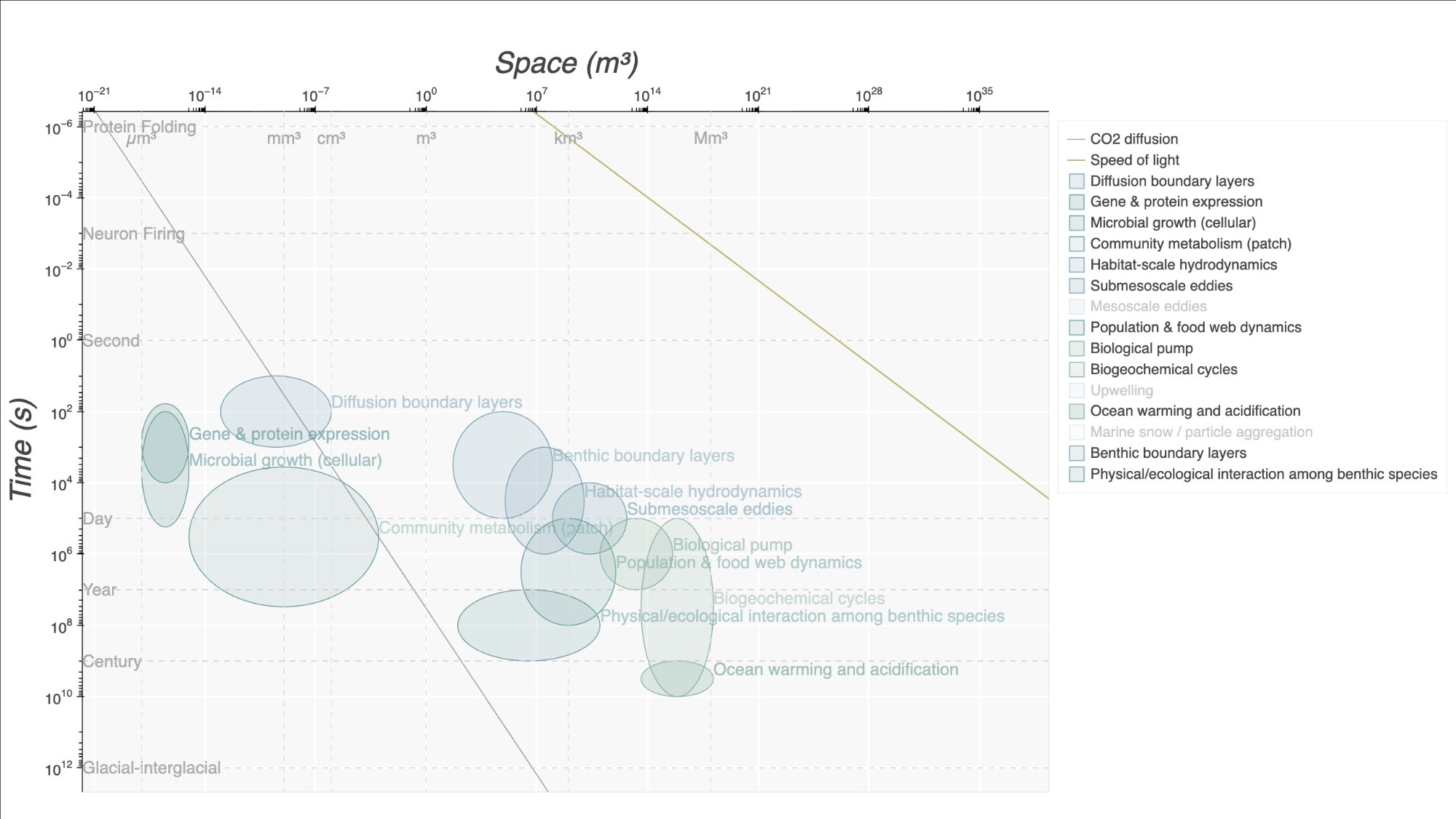
timeSpace plots processes and reference objects on log-log Stommel diagrams — a visualization framework where the x-axis represents spatial scale (m³) and the y-axis represents temporal scale (s), as shown in Boyd et al. (2015) Fig. 1. See CONVENTIONS.md for details on axis orientation and units. Processes are rendered as ellipses sized to their characteristic ranges, with diffusion lines overlaid to show transport regimes. This makes it easy to see which processes dominate at which scales and how they relate to one another.

Install

pip install timeSpace            # core (Bokeh diagrams)
pip install timeSpace[dev]       # + pytest, black, flake8

Note: PyPI normalizes the package name to timespace, but the Python import uses camelCase: import timeSpace.

Quickstart

import timeSpace
import pandas as pd
from timeSpace import (
    create_space_time_figure,
    add_magnitude_labels,
    add_diffusion_lines,
    add_light_cone,
    add_predefined_processes,
    add_legend,
)
from timeSpace.etl import transform_predefined_processes

# Load bundled process data
csv_path = timeSpace.PROJECT_ROOT / "data" / "datasets" / "stommel_boyd2015_volumes.csv"
data = pd.read_csv(csv_path)
df = transform_predefined_processes(data)

# Build the diagram
p = create_space_time_figure()
p = add_magnitude_labels(p)
p = add_diffusion_lines(p)
p = add_light_cone(p)
p = add_predefined_processes(p, df)
p = add_legend(p)

from bokeh.plotting import show
show(p)

For a worked example, see the desert farm Stommel diagram notebook.

Conventions

See CONVENTIONS.md for details on axis orientation (Boyd vs. classic Stommel), volume units (m³) for spatial scale, the diffusion equation (3D RMS: √(6Dt)), and data file schemas.

Data Format

All spatial values are volumes in m³ (not lengths). All temporal values are durations in seconds. Both axes are plotted on log₁₀ scales.

CSV columns for process data:

• Required: Name, Time_min, Time_max, Space_min, Space_max
• Optional: Color, Category, Notes, label_side, x_offset, y_offset, label_text

Values use scientific notation with an optional magnitude description, e.g. 1.00E-03: ~1 mm³. The ETL layer parses the numeric portion before the colon; the description is for human readability.

See CONVENTIONS.md for the full schema specification.

Plotting Functions: add_processes vs add_predefined_processes

Use add_predefined_processes(p, df) for the bundled Boyd (2015) dataset — it expects data from transform_predefined_processes() with pre-assigned colors and categories.

Use add_processes(p, df) for your own data — it supports grouping, custom colors via category_col and category_colors, and per-row label_side control. Expects data from transform_process_response_sheet().

# Bundled dataset
from timeSpace.etl import transform_predefined_processes
df = transform_predefined_processes(pd.read_csv(csv_path))
p = add_predefined_processes(p, df)

# Your own data
from timeSpace.etl import transform_process_response_sheet
df = transform_process_response_sheet(my_data)
p = add_processes(p, df, category_col="category_type", category_colors={"Physical": "#7BA3B3"})

Google Sheets Integration

timeSpace can pull process and measurement data directly from Google Sheets, which is useful for collaborative data entry via Google Forms.

Using Google Sheets with pip install

If you installed via pip (no git clone), you can fetch sheet data directly:

from timeSpace import extract_google_sheet
from timeSpace.etl import transform_process_response_sheet

df = extract_google_sheet(spreadsheet_id="YOUR_SHEET_ID", data_name="processes")
processed = transform_process_response_sheet(df)

Setting up a processes form

1. Use this link to create your own copy of the processes Google Form
2. After renaming the form / updating the description and questions, go to the Responses tab and click "Link to Sheets"
3. Update the permissions on the newly created sheet to be viewable by anyone with the link
4. Copy the sheet URL
5. In constants.py, set PROCESSES_URI to the identifying string between /d/ and /edit in the sheet URL. For example: https://docs.google.com/spreadsheets/d/USE_THIS_PART/edit?gid=0#gid=0

Editing the Time / Space scale answer options

The scale answer options in the form follow the format <value>: <example>, for instance 1.00E+07: ~3 months.

• The numeric value before the : (e.g. 1.00E+07) is what the ETL parses and plots. Do not change these — the code (etl.py) splits on : and casts the prefix to float, so anything non-numeric or out of the expected decade will break downstream processing or silently shift your data.
• The example text after the : (e.g. ~3 months) is purely a human-readable anchor. You can edit it freely to make the scale more intuitive for your respondents.

Setting up a measurement form

Follow the same steps as above, using your measurement form template, and set MEASUREMENTS_URI in constants.py.

Setting up predefined processes

1. Create your own copy of the predefined processes Google Sheet
2. Update permissions so the sheet is viewable by anyone with the link
3. Set PREDEFINED_PROCESSES_URI in constants.py to the sheet ID

Using Google Sheets data in code

from timeSpace.data_processing import extract_google_sheet
from timeSpace.etl import transform_process_response_sheet

# Fetch sheet data (caches locally as CSV)
df = extract_google_sheet(spreadsheet_id="YOUR_SHEET_ID", data_name="processes")
processed = transform_process_response_sheet(df)

Bokeh Output Modes

timeSpace uses Bokeh for rendering. There are three main ways to display or save diagrams:

• show(p) — opens the diagram in your default browser with full interactivity (hover, zoom, pan).
• output_file("diagram.html") + save(p) — writes a self-contained static HTML file.
• components(p) — returns (script, div) HTML strings for embedding in your own page or iframe. Use this for embedding in Google Sites or other CMS platforms (see docs/explorer.html for an example).

from bokeh.plotting import output_file, save, show
from bokeh.embed import components

# Interactive in browser
show(p)

# Save to file
output_file("stommel.html")
save(p)

# Embed in another page
script, div = components(p)

Data files

Bundled CSV data in data/datasets/:

• stommel_boyd2015_volumes.csv — process definitions (time/space ranges, categories) used for the default Stommel diagram
• time_space_reference_objects.csv — 102 reference objects across 10 categories for scale context

Development

git clone https://github.com/MDunitz/timeSpace.git
cd timeSpace
pip install -e ".[dev]"
pytest tests/

Public API

All key functions are importable directly from timeSpace:

from timeSpace import (
    # Plotting
    create_space_time_figure,  # Create the base log-log Stommel figure
    add_magnitude_labels,      # Add time/space scale reference lines and labels
    add_processes,             # Add custom process ellipses (from user data)
    add_predefined_processes,  # Add processes from bundled CSV
    add_diffusion_lines,       # Overlay molecular diffusion curves
    add_light_cone,            # Add speed-of-light causality boundary
    add_legend,                # Move legend to right panel with toggle

    # Measurements
    add_measurements,          # Add measurement scatter points with labels
    add_grouped_measurement,   # Add measurements grouped by field (e.g. lab)

    # Calculations
    create_ellipse_data,          # Generate ellipse polygon vertices in log space
    calculate_diffusion_length,   # L = sqrt(4Dt/π), returns astropy Quantity
    calculate_sphere_volume,      # V = (4/3)πr³, returns astropy Quantity
    classify_process_geometry,    # Detect degenerate axes → ellipse/line/point

    # Label placement
    resolve_label_overlaps,  # Force-directed label collision resolution
    count_overlaps,          # Count remaining label overlaps after placement

    # ETL
    transform_process_response_sheet,  # Clean Google Form responses
    transform_predefined_processes,    # Prepare bundled CSV for plotting
    transform_measurement_sheet,       # Clean measurement form responses

    # Data access
    extract_google_sheet,  # Fetch data from Google Sheets (with local CSV cache)
)