The goal of this project is to identify frogs, deer, and trucks by using various neural net models. These models include CNN, VNN, and MC dropout. I will try and identify interesting cases from each of the three models.
library(keras) library(tensorflow) library(pROC) library(magick) library(viridis)
tf$compat$v1$disable_eager_execution()
K <- backend()
if (tensorflow::tf$executing_eagerly()) tensorflow::tf$compat$v1$disable_eager_execution()
load('deers_frogs_trucks.Rdata')
img_rows <- 32 img_cols <- 32
input_shape <- c(img_rows, img_cols, 3)
num_classes <- 3
cat('x_train_shape:', dim(x_train), '\n')
cat(nrow(x_train), 'train samples\n')
cat(nrow(x_test), 'test samples\n')
I loaded the packages and imported the data set for this project in the above chunk along with specifying the input_shape and the number of classes for the models. The number of classes was set to three because there are three different types of images in this data set.
The first model I looked at was the CNN model.
Define the model.
inputs = layer_input(shape = input_shape)
model <- keras_model_sequential() %>% layer_conv_2d(filters = 32, kernel_size = c(3,3), activation = 'relu', input_shape = input_shape) %>% layer_max_pooling_2d(pool_size = c(2, 2)) %>% layer_conv_2d(filters = 64, kernel_size = c(3,3), activation = 'relu',name='Conv_last') %>% layer_max_pooling_2d(pool_size = c(2, 2)) %>% layer_flatten() %>% layer_dense(units = 128, activation = 'relu') %>% layer_dropout(rate = 0.2) %>% layer_dense(units = 128, activation = 'relu') %>% layer_dropout(rate = 0.2) %>% layer_dense(units = num_classes, activation = 'softmax')
summary(model)
In this step I defined the CNN model with two convolutional layers and two max pooling layers. The first convolutional layer had 32 filters with a 3x3 kernel, while the second layer had 64 filters and a 3x3 kernel. Each of the max pooling layers had a pooling size of 2x2. These layers were followed by a flatten layer and three dense layers. These dense layers had 128 units and a relu activation. The last dense layer used the number of classes as the number of units and had a softmax activation because we were dealing with multiple categories for classification. The model ended up having 331,331 total parameters.
Specify optimizer, loss function, metrics, set up early stopping, and run the optimization.
model %>% compile( loss = 'categorical_crossentropy', optimizer = 'adam', metrics = c('accuracy') )
callback_specs=list(callback_early_stopping(monitor = "val_loss", min_delta = 0, patience = 10, verbose = 0, mode = "auto"), callback_model_checkpoint(filepath='best_model.hdf5',save_freq='epoch' ,save_best_only = TRUE) )
history <- model %>% fit( x_train, y_train, epochs = 50, batch_size = 256, validation_split = 0.2, callbacks = callback_specs )
I specified the loss function as categorical_crossentropy and the metric as accuracy because we are categorizing the images. I set up an early stopping function to make sure the model was not over fit. Lastly, the model was fit using the train and test data with a 20% validation split. We used 256 batches to improve the accuracy on the test data along with 50 epochs. These specifications helped improve the performance of the model.
Calculate the accuracy and area under the curve of the model.
model_best = load_model_hdf5('best_model.hdf5',compile=TRUE)
model_best %>% evaluate(x_test,y_test)
p_hat_test = model_best %>% predict(x_test) y_hat_test = apply(p_hat_test,1,which.max)
model %>% evaluate(x_test, y_test)
y_true = apply(y_test,1,which.max) sum(y_hat_test==y_true)/length(y_true)
multiclass.roc(y_true,y_hat_test)
model %>% evaluate(x_test, y_test)
sum(y_hat_test==y_true)/length(y_true)
multiclass.roc(y_true,y_hat_test)
After running the above code we can see that the model had an accuracy of around 91% and a AUC of 0.94. These are really solid results for this model. In the future increasing the epochs might yield better results but for now this model is good.
Use grad CAM method to analyze the 11th picture.
test_case_to_look <- 11 # Case 11 number_of_filters <- 64 # Number of filers for last layer
last_conv_layer <- model_best %>% get_layer("Conv_last")
target_output <- model_best$output[, which.max(y_test[test_case_to_look,])]
grads <- K$gradients(target_output, last_conv_layer$output)[[1]]
pooled_grads <- K$mean(grads, axis = c(1L, 2L))
compute_them <- K$function(list(model_best$input),
list(pooled_grads, last_conv_layer$output[1,,,]))
x_test_example <- x_test[test_case_to_look,,,] dim(x_test_example) <- c(1,dim(x_test_example))
which.max(y_test[test_case_to_look,])
which.max(model_best %>% predict(x_test_example))
c(pooled_grads_value, conv_layer_output_value) %<-% compute_them(list(x_test_example))
for (i in 1:number_of_filters) { conv_layer_output_value[,,i] <- conv_layer_output_value[,,i] * pooled_grads_value[[i]] }
heatmap <- apply(conv_layer_output_value, c(1,2), mean)
heatmap <- pmax(heatmap, 0) heatmap <- (heatmap - min(heatmap))/ (max(heatmap)-min(heatmap))
write_heatmap <- function(heatmap, filename, width = 32, height = 32, bg = "white", col = terrain.colors(12)) { png(filename, width = width, height = height, bg = bg) op = par(mar = c(0,0,0,0)) on.exit({par(op); dev.off()}, add = TRUE) rotate <- function(x) t(apply(x, 2, rev)) image(rotate(heatmap), axes = FALSE, asp = 1, col = col) }
image <- image_read(x_test[test_case_to_look,,,]) info <- image_info(image) geometry <- sprintf("%dx%d!", info$width, info$height)
pal <- col2rgb(viridis(20), alpha = TRUE) alpha <- floor(seq(0, 255, length = ncol(pal))) pal_col <- rgb(t(pal), alpha = alpha, maxColorValue =255) write_heatmap(heatmap, "overlay.png", width = 32, height = 32, bg = NA, col = pal_col)
par(mfrow=c(1,2)) image %>% plot() image_read("overlay.png") %>% image_resize(geometry, filter = "quadratic") %>% image_composite(image, operator = "blend", compose_args = "35") %>% plot()
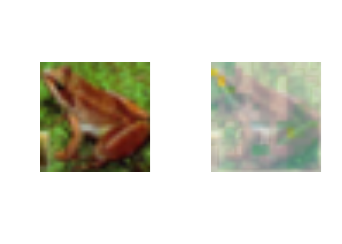
Looking at this image we can tell it is of a frog. This model identifies the image as a frog by looking at the area around its eye and the space between its legs. I thought this was really cool to see how big of an impact the indentation of the frogs eye had on the classification posses.
Use grad CAM method to analyze the 13th picture.
test_case_to_look <- 13 # Case 13 number_of_filters <- 64 # Number of filers for last layer
last_conv_layer <- model_best %>% get_layer("Conv_last")
target_output <- model_best$output[, which.max(y_test[test_case_to_look,])]
grads <- K$gradients(target_output, last_conv_layer$output)[[1]]
pooled_grads <- K$mean(grads, axis = c(1L, 2L))
compute_them <- K$function(list(model_best$input),
list(pooled_grads, last_conv_layer$output[1,,,]))
x_test_example <- x_test[test_case_to_look,,,] dim(x_test_example) <- c(1,dim(x_test_example))
which.max(y_test[test_case_to_look,])
which.max(model_best %>% predict(x_test_example))
c(pooled_grads_value, conv_layer_output_value) %<-% compute_them(list(x_test_example))
for (i in 1:number_of_filters) { conv_layer_output_value[,,i] <- conv_layer_output_value[,,i] * pooled_grads_value[[i]] } heatmap <- apply(conv_layer_output_value, c(1,2), mean)
heatmap <- pmax(heatmap, 0) heatmap <- (heatmap - min(heatmap))/ (max(heatmap)-min(heatmap))
write_heatmap <- function(heatmap, filename, width = 32, height = 32, bg = "white", col = terrain.colors(12)) { png(filename, width = width, height = height, bg = bg) op = par(mar = c(0,0,0,0)) on.exit({par(op); dev.off()}, add = TRUE) rotate <- function(x) t(apply(x, 2, rev)) image(rotate(heatmap), axes = FALSE, asp = 1, col = col) }
image <- image_read(x_test[test_case_to_look,,,]) info <- image_info(image) geometry <- sprintf("%dx%d!", info$width, info$height)
pal <- col2rgb(viridis(20), alpha = TRUE) alpha <- floor(seq(0, 255, length = ncol(pal))) pal_col <- rgb(t(pal), alpha = alpha, maxColorValue =255) write_heatmap(heatmap, "overlay.png", width = 32, height = 32, bg = NA, col = pal_col)
par(mfrow=c(1,2)) image %>% plot() image_read("overlay.png") %>% image_resize(geometry, filter = "quadratic") %>% image_composite(image, operator = "blend", compose_args = "35") %>% plot()
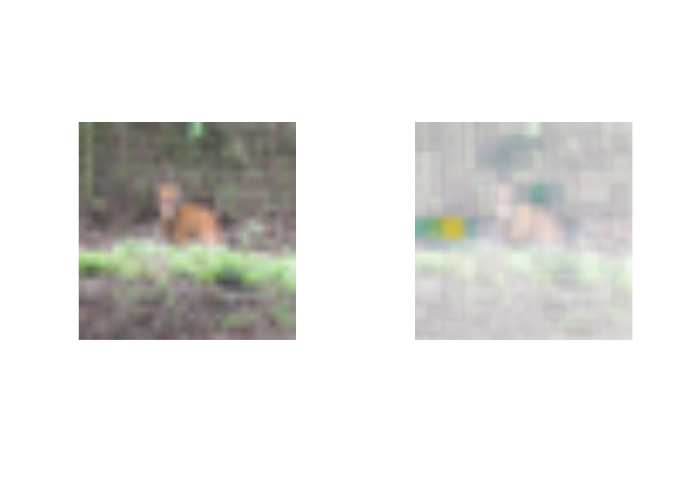
The second case I wanted to look at was of a deer standing in the woods. I thought it was interesting and maybe troubling that the model used the woods next to the deer to categorize the image. I feel like this case might not have the best results since the model focused on the background of the image.
Use grad CAM method to analyze the 17th picture.
test_case_to_look <- 17 # Case 17 number_of_filters <- 64 # Number of filers for last layer
last_conv_layer <- model_best %>% get_layer("Conv_last")
target_output <- model_best$output[, which.max(y_test[test_case_to_look,])]
grads <- K$gradients(target_output, last_conv_layer$output)[[1]]
pooled_grads <- K$mean(grads, axis = c(1L, 2L))
compute_them <- K$function(list(model_best$input),
list(pooled_grads, last_conv_layer$output[1,,,]))
x_test_example <- x_test[test_case_to_look,,,] dim(x_test_example) <- c(1,dim(x_test_example))
which.max(y_test[test_case_to_look,])
which.max(model_best %>% predict(x_test_example))
c(pooled_grads_value, conv_layer_output_value) %<-% compute_them(list(x_test_example))
for (i in 1:number_of_filters) { conv_layer_output_value[,,i] <- conv_layer_output_value[,,i] * pooled_grads_value[[i]] } heatmap <- apply(conv_layer_output_value, c(1,2), mean)
heatmap <- pmax(heatmap, 0) heatmap <- (heatmap - min(heatmap))/ (max(heatmap)-min(heatmap))
write_heatmap <- function(heatmap, filename, width = 32, height = 32, bg = "white", col = terrain.colors(12)) { png(filename, width = width, height = height, bg = bg) op = par(mar = c(0,0,0,0)) on.exit({par(op); dev.off()}, add = TRUE) rotate <- function(x) t(apply(x, 2, rev)) image(rotate(heatmap), axes = FALSE, asp = 1, col = col) }
image <- image_read(x_test[test_case_to_look,,,]) info <- image_info(image) geometry <- sprintf("%dx%d!", info$width, info$height)
pal <- col2rgb(viridis(20), alpha = TRUE) alpha <- floor(seq(0, 255, length = ncol(pal))) pal_col <- rgb(t(pal), alpha = alpha, maxColorValue =255) write_heatmap(heatmap, "overlay.png", width = 32, height = 32, bg = NA, col = pal_col)
par(mfrow=c(1,2)) image %>% plot() image_read("overlay.png") %>% image_resize(geometry, filter = "quadratic") %>% image_composite(image, operator = "blend", compose_args = "35") %>% plot()
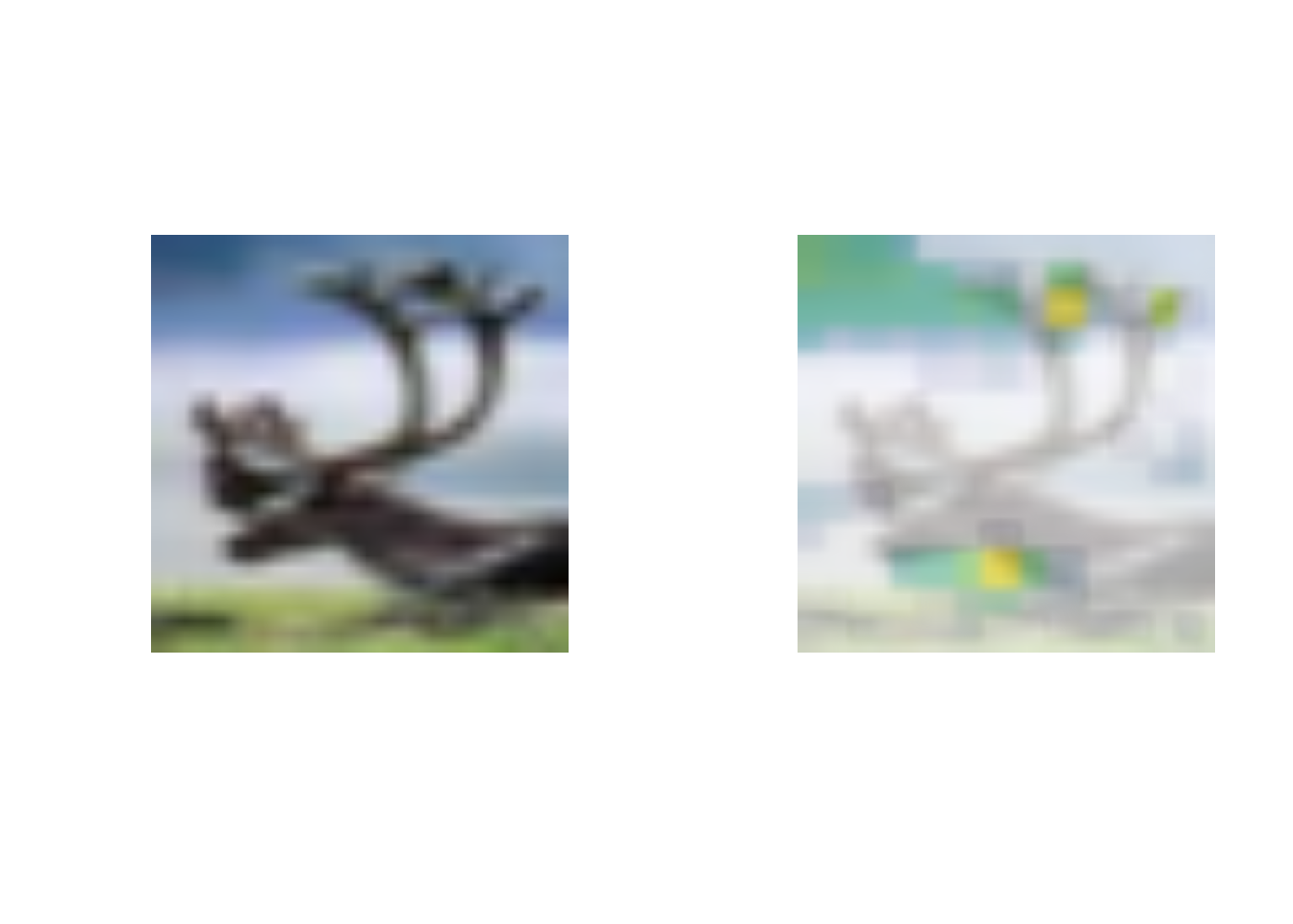
The last picture I wanted to look at using the CNN method and utilizing grad CAM was the 17th case. This image was of a deers head and antlers. The model focused heavily of the tips of the antlers which seems like a natural feature to look at. It seems the model had a much easier time identifying this image as a deer opposed to the last case.
The second model I looked at was the VNN model.
Define the model and its parameters.
batch_size <- 100L latent_dim <- 32L intermediate_dim <- 64L epochs <- 75L epsilon_std <- 1.0
input_shape <- c(img_rows, img_cols, 3)
x <- layer_input(shape = input_shape) h <- layer_conv_2d(x,filters = 32, kernel_size = c(3,3), activation = 'relu', padding='same') %>% layer_max_pooling_2d(pool_size = c(2, 2)) %>% layer_conv_2d(filters = 64, kernel_size = c(3,3), activation = 'relu') %>% layer_max_pooling_2d(pool_size = c(2, 2)) %>% layer_flatten() %>% layer_dense(intermediate_dim, activation = "relu") %>% layer_dense(intermediate_dim, activation = "relu") z_mean <- layer_dense(h, latent_dim) z_log_var <- layer_dense(h, latent_dim) sampling <- function(arg){ z_mean <- arg[, 1:(latent_dim)] z_log_var <- arg[, (latent_dim + 1):(2 * latent_dim)] epsilon <- k_random_normal( shape = c(k_shape(z_mean)[[1]]), mean=0., stddev=epsilon_std ) z_mean + k_exp(z_log_var/2)*epsilon }
z <- layer_concatenate(list(z_mean, z_log_var)) %>% layer_lambda(sampling)
decoder_h <- layer_dense(units = intermediate_dim, activation = "relu") decoder_p <- layer_dense(units = 3, activation = 'softmax') h_decoded <- decoder_h(z) y_decoded_p <- decoder_p(h_decoded)
vnn <- keras_model(x, y_decoded_p)
encoder <- keras_model(x, z_mean)
The model was run using 75 epochs, a latent dimension of 32, and an intermediate dimension of 64. The input layer for the model was the same as the last model and was saved as x. Two convolutional layers with 32 and 64 filters were used with a 3x3 kernel. Like the CNN model, each of the model had two max pooling layers with a pooling size of 2x2. These were followed by two dense layers with the activation function relu. THe next two layers contained the latent dimension for the model. Later on the model was decoded using the intermediate dimension with relu activation in a dense layer. This was followed by another dense layer with three units and the softmax activation. This was then saved as the vnn model.
Specify optimizer, loss function, metrics, set up early stopping, and run the optimization.
vnn_loss <- function(x, x_decoded_mean){ cat_loss <- loss_categorical_crossentropy(x, x_decoded_mean) kl_loss <- -0.5*k_mean(1 + z_log_var - k_square(z_mean) - k_exp(z_log_var), axis = -1L) cat_loss + kl_loss }
vnn %>% compile(optimizer = "adam", loss = vnn_loss, metrics = c('accuracy'))
vnn %>% fit( x_train, y_train, shuffle = TRUE, epochs = epochs, batch_size = batch_size, validation_data = list(x_train,y_train) )
I specified the cat_loss as loss_categorical_crossentropy and the metric as accuracy because we are categorizing the images. The model was fit using the train and test data with a validation split defined by these data sets. The vnn loss function was used in the compile function for the loss. I used the defined number of batches and epochs to run the model.
Calculate the accuracy and area under the curve of the model.
vnn %>% evaluate(x_test,y_test)
p_hat_test = vnn %>% predict(x_test) y_hat_test = apply(p_hat_test,1,which.max)
vnn %>% evaluate(x_test, y_test)
y_true = apply(y_test,1,which.max) sum(y_hat_test==y_true)/length(y_true)
multiclass.roc(y_true,y_hat_test)
vnn %>% evaluate(x_test, y_test)
sum(y_hat_test==y_true)/length(y_true)
multiclass.roc(y_true,y_hat_test)
After running the above code we can see that the model had an accuracy of around 88% and a AUC of 0.92. Again, these are really solid. In the future the latent dimension could be experimented with in order to achieve better results.
Predict the values from the model and examine cases.
x_test_decoded <- array(NA,dim=c(3000,3,1000)) for(i in 1:1000) { x_test_decoded[,,i] <- predict(vnn, x_test) }
par(mfrow=c(1,2))
test_case_to_look <- 18 image <- image_read(x_test[test_case_to_look,,,]) image %>% plot()
prob_to_plot <- t(x_test_decoded[18,,]) boxplot(prob_to_plot)
par(mfrow=c(1,2))
test_case_to_look <- 24 image <- image_read(x_test[test_case_to_look,,,]) image %>% plot()
prob_to_plot <- t(x_test_decoded[24,,]) boxplot(prob_to_plot)
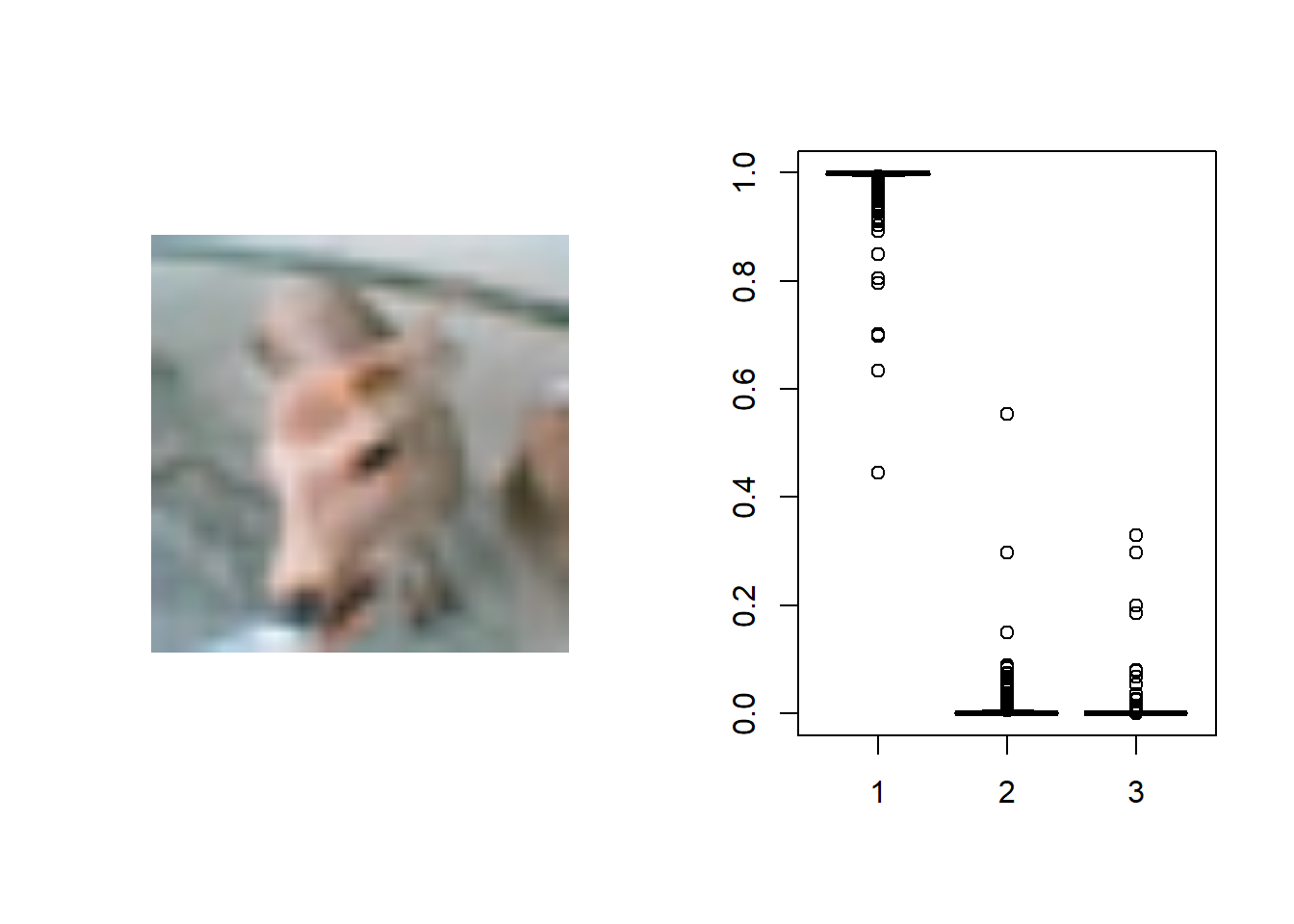
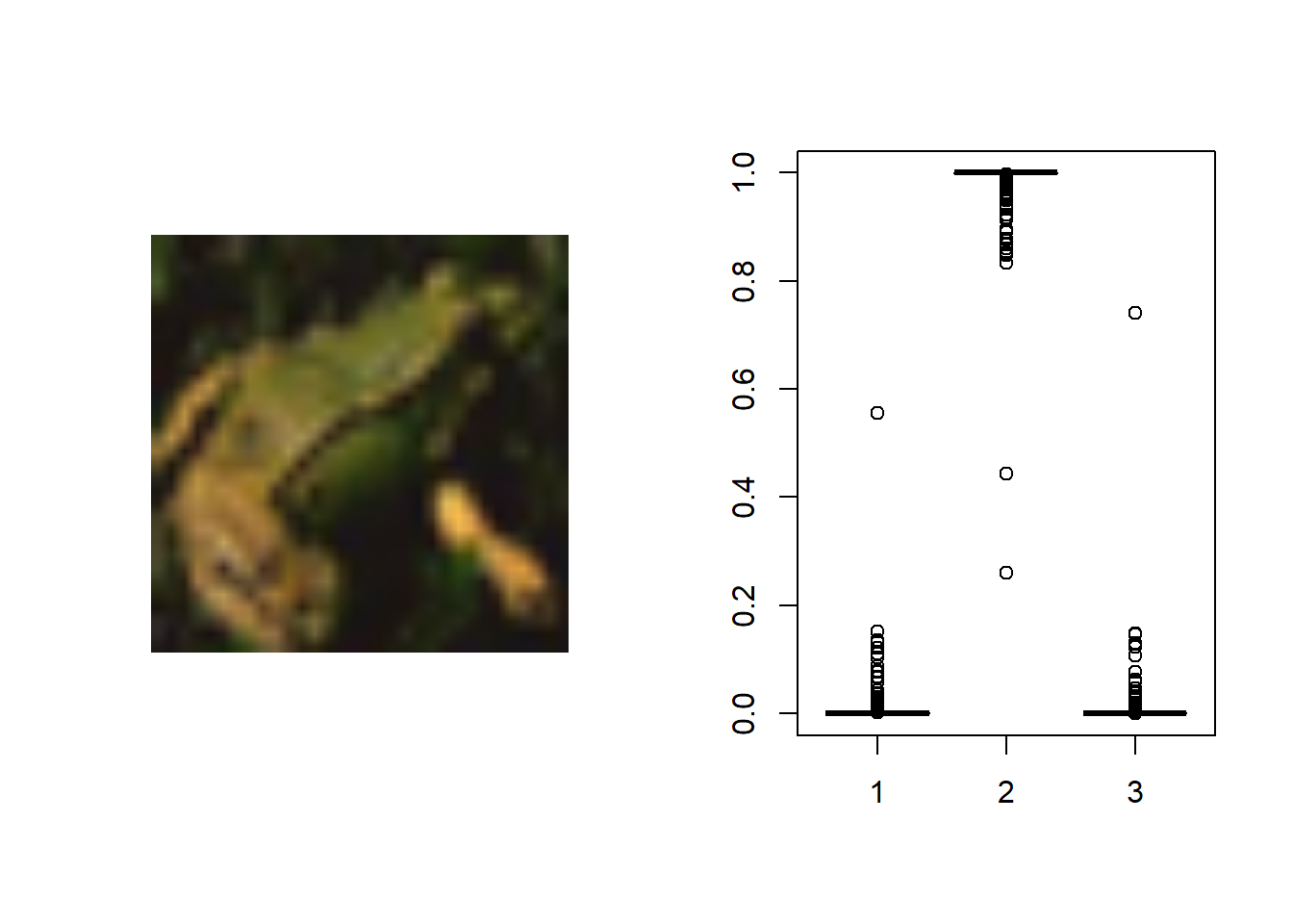
In this code the values were predicted by looping over the test data and the vnn model 1000 times. These values were then applied to image 18 and 24. In case 18 the model correctly identified a frog but in case 24 the model mistakenly identified the deer as a frog. I think the misclassification happened because the image is manly of the deers head, making the model miss the bigger picture.
The third model I looked at was the MC dropout model.
Define the model and its parameters.
DropoutRate <- 0.5 tau <- 0.5 keep_prob <- 1-DropoutRate n_train <- nrow(x_train) penalty_weight <- keep_prob/(tau* n_train) penalty_intercept <- 1/(tau* n_train)
dropout_1 <- layer_dropout(rate = DropoutRate) dropout_2 <- layer_dropout(rate = DropoutRate)
input_shape <- c(img_rows, img_cols, 3)
inputs = layer_input(shape = input_shape) output <- inputs %>% layer_conv_2d(filters = 32, kernel_size = c(3,3), activation = 'relu') %>% layer_max_pooling_2d(pool_size = c(2, 2)) %>% layer_conv_2d(filters = 64, kernel_size = c(3,3), activation = 'relu') %>% layer_max_pooling_2d(pool_size = c(2, 2)) %>% layer_conv_2d(filters = 128, kernel_size = c(3,3), activation = 'relu') %>% layer_max_pooling_2d(pool_size = c(2, 2)) %>% layer_flatten() %>% layer_dense(units = 128, activation = 'relu', kernel_regularizer=regularizer_l2(penalty_weight), bias_regularizer=regularizer_l2(penalty_intercept)) %>% dropout_1(training=TRUE) %>% layer_dense(units = 64, activation = 'relu', kernel_regularizer=regularizer_l2(penalty_weight), bias_regularizer=regularizer_l2(penalty_intercept)) %>% dropout_2(training=TRUE) %>% layer_dense(units = 3, activation = 'softmax', kernel_regularizer=regularizer_l2(penalty_weight), bias_regularizer=regularizer_l2(penalty_intercept)) model <- keras_model(inputs, output)
summary(model)
The input layer for the model was the same as the first model. The dropout rate was defined as 0.5 with a tau of 0.5. Two dropout layers were defined using the rate. The output layer contained three convolutional layers with 32, 64, and 128 filters respectively. Each had a kernel of 3x3. Like the CNN model, the model contained max pooling layers with a pooling size of 2x2. These were followed by dense layers with the activation function relu and the two dropout layers. The final dense layer had the softmax activation layer and three units. This was because there are three different categories we are classifying. This model had 167,363 total parameters.
Specify optimizer, loss function, metrics, set up early stopping, and run the optimization.
model %>% compile( loss = 'categorical_crossentropy', optimizer = 'adam', metrics = c('accuracy') )
callback_specs=list(callback_early_stopping(monitor = "val_loss", min_delta = 0, patience = 10, verbose = 0, mode = "auto"), callback_model_checkpoint(filepath='best_model.hdf5',save_freq='epoch' ,save_best_only = TRUE) )
history <- model %>% fit( x_train, y_train, epochs = 50, batch_size = 200, validation_split = 0.2, callbacks = callback_specs )
I specified the loss function as categorical_crossentropy and the metric as accuracy because we are categorizing the images. I set up an early stopping function to make sure the model was not over fit. Lastly, the model was fit using the train and test data with a 20% validation split. We used 200 batches to improve the accuracy on the test data along with 50 epochs. These specifications helped improve the performance of the model.
Calculate the accuracy and area under the curve of the model.
model_best = load_model_hdf5('best_model.hdf5',compile=TRUE)
model_best %>% evaluate(x_test,y_test)
p_hat_test = model_best %>% predict(x_test) y_hat_test = apply(p_hat_test,1,which.max)
model_best %>% evaluate(x_test, y_test)
y_true = apply(y_test,1,which.max) sum(y_hat_test==y_true)/length(y_true) #### do we get the same result?
multiclass.roc(y_true,y_hat_test)
model_best %>% evaluate(x_test, y_test)
sum(y_hat_test==y_true)/length(y_true)
multiclass.roc(y_true,y_hat_test)
After running the above code we can see that the model had an accuracy of around 90% and a AUC of 0.93. Again, these are really solid. The number of epochs could be increased to possibly raise the accuracy of the model. Furthermore, after decreasing the dropout rate the model appeared to have a more difficult time classifying images. The accuracy of the model was not quite as high as it is now but this might be worth revisiting in the future.
Predict the values from the model and examine cases.
mc.sample=1000
testPredict=array(NA,dim=c(nrow(x_test),3,mc.sample)) for(i in 1:mc.sample) { testPredict[,,i]=model_best %>% predict(x_test) }
par(mfrow=c(1,2))
test_case_to_look <- 16 image <- image_read(x_test[test_case_to_look,,,]) image %>% plot()
prob_to_plot <- t(testPredict[16,,]) boxplot(prob_to_plot)

par(mfrow=c(1,2))
test_case_to_look <- 17 image <- image_read(x_test[test_case_to_look,,,]) image %>% plot()
prob_to_plot <- t(testPredict[17,,]) boxplot(prob_to_plot)
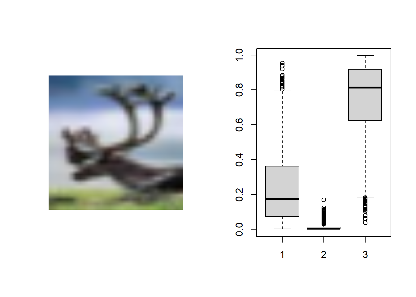
In this code the values were predicted by looping over the test data and the model best 1000 times. These values were then applied to image 16 and 17. In case 16 the model correctly identified a truck without a doubt but in case 17 the model mistakenly identified the deer as a truck. The model appeared to think the deer was a truck with a possibility that it could be a deer. I thought this was interesting that the same picture of the deer was distinctly identified using grad CAM but in this model it thinks it could be a truck. I noticed throughout the models they seemed to be really good at identifying trucks but not so good at identifying deer. I can understand why trucks might be easier to identify because they have a lot of straight lines vs deer who do not have as distinct features (ones without antlers). This was a really interesting case study that deserves more attention in the future.